Causal Inference Variance Reduction with Precision Variables
In causal inference, covariates that correlate with the outcome but remain independent of the treatment can be used to reduce the standard error of causal effect estimates. These variables are known as precision variables.
This note demonstrates the mechanism behind standard error reduction using precision variables through numerical simulation and mathematical derivation.
Precision Variables
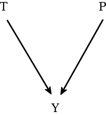
Figure 1 shows a directed acyclic graph (DAG) of the causal relationship among the variables $T$, $P$, and $Y$. We want to estimate the effect of the treatment $T$ on the outcome $Y$.
The variable $P$ qualifies as a precision variable if it satisfies two conditions:
- Independence from treatment: $P\perp T$ and $\text{Cov}(T, P)=0$. Including $P$ does not alter the expected value (unbiasedness) of the treatment effect estimate.
- Association with the outcome: The variable P explains a non-zero portion of the variability in Y conditional on $T$, such that $\text{Cov}(P, Y) \neq 0$.
Including a precision variable $P$ in the regression model reduces the residual variance of the outcome, which directly decreases the standard error of the estimated treatment coefficient without introducing bias.
Numerical Simulations
To illustrate this effect, we evaluate three linear simulation scenarios.
Case 1: One Precision Variable $P$ Which Directly Affects $Y$
The linear data-generating process is defined as:
\[Y = 1 + 2*T + 3*P + \epsilon, \notag\]where $\epsilon$ represents random noise such that $\epsilon \sim \mathcal{N}(0,1)$.
The table below summarizes the results for models with and without the precision variable. The standard error of the treatment coefficient decreases by $ 67.9\%$ when the precision variable is added. Additionally, the $R^2$ increases substantially while the RMSE drops.
| Model | Coefficient | Standard Error (SE) | SE Reduction (%) | $R^2$ | RMSE |
|---|---|---|---|---|---|
| $Y \sim T$ | 2.23 | 0.197 | 0.11 | 3.11 | |
| $Y \sim T + P$ | 2.02 | 0.0633 | 67.9% | 0.91 | 0.99 |
Case 2: Two Precision Variables $P_1$ and $P_2$ Which Directly Affect $Y$
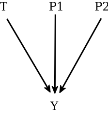
In this case, there are two independent precision variables, as shown in Figure 2. The data-generating process is:
\[Y = 1 + 2*T + 2.5*P_1 + 1.8 P_2 + \epsilon, \notag\]where $\epsilon \sim \mathcal{N}(0,1)$.
As shown in the table, incorporating multiple precision variables yields an accumulative reduction in the standard error of the treatment effect
| Model | Coefficient | Standard Error (SE) | SE Reduction (%) | $R^2$ | RMSE |
|---|---|---|---|---|---|
| $Y \sim T$ | 2.25 | 0.201 | 0.11 | 3.18 | |
| $Y \sim T + P_1$ | 2.08 | 0.132 | 34.5% | 0.62 | 2.07 |
| $Y \sim T + P_2$ | 2.23 | 0.171 | 15.1% | 0.36 | 2.69 |
| $Y \sim T + P_1 + P_2$ | 2.05 | 0.0655 | 67.5% | 0.91 | 1.03 |
Case 3: One Precision Variable $P$ Which Shares a Confounder with $Y$
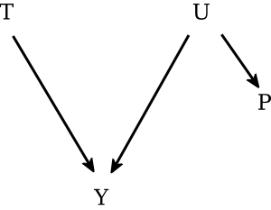
The data generating process is given by:
\[\begin{align} \notag Y & = 1 + 2 T + 2.5 U + \epsilon, \\ \notag P & = 1.5 U + \delta \notag, \end{align}\]where $U$ is an unobserved common cause of $P$ and $Y$, with $\epsilon \sim \mathcal{N}(0,1)$ and $\delta \sim \mathcal{N}(0,1)$.
Controlling for proxy precision variables that share confounders with the outcome also successfully reduces the standard error of the treatment coefficient and improves overall model fit.
| Model | Coefficient | Standard Error (SE) | SE Reduction (%) | $R^2$ | RMSE |
|---|---|---|---|---|---|
| $Y \sim T$ | 1.92 | 0.172 | 0.11 | 2.72 | |
| $Y \sim T + P$ | 1.98 | 0.0822 | 52.2% | 0.80 | 1.30 |
Derivation in the Linear Case
The following mathematical derivation proves why a precision variable reduces the standard error of the estimated treatment effect coefficient.
By definition of the precision variable:
-
$T\perp P$: $\text{Cov}(T, P)=0$.
-
$P$ and $Y$ are correlated: $\text{Cov}(Y, P) \neq 0$ (whether through a direct path or shared confounder).
-
$P$ exhibits a non-constant distribution: $\text{Var}(P) >0$.
Assume the true population data-generating process for independent observations is linear:
\[Y_i = \beta_0 + \beta_1 T_i + \beta_2 P_i + \epsilon_i \label{true_model}\]When regressing $Y$ on $T$ alone, the unadjusted model is:
\[Y_i = \alpha_0 + \beta_{\text{unadj}} T_i + \epsilon_i. \label{unadjusted_model_orig}\]Taking the covariance of both sides of the Equation ($\ref{unadjusted_model}$) with $T$ yields:
\[\beta_{\text{unadj}} = \frac{\text{Cov}(Y, T)}{\text{Var}(T)}. \notag\]From Equation ($\ref{true_model}$), we expand the numerator:
\[\text{Cov}(Y, T) = \beta_1\text{Var}(T) + \beta_2\text{Cov}(P, T)=\beta_1\text{Var}(T),\notag\]since $\text{Cov}(P, T) = 0$. Therefore $\beta_{\text{unadj}} = \beta_1$, meaning Equation ($\ref{unadjusted_model_orig}$) simplifies to:
\[Y_i = \alpha_0 + \beta_1 T_i + \epsilon_i. \label{unadjusted_model}\]From Equations ($\ref{true_model}$ and $\ref{unadjusted_model}$), the error term $\delta_i$ satisfies:
\[\delta_i = \beta_0 + \beta_2 P_i + \epsilon_i - \alpha_0. \label{delta}\]Taking the population average of Equations ($\ref{true_model}$ and $\ref{unadjusted_model}$) gives:
\[E(Y) = \beta_0 + \beta_1 E(T) + \beta_2 E(P) \\ \label{expectation_true}\] \[E(Y) = \alpha_0 + \beta_1 E(T) \label{expectation_unadjusted}\]Equating ($\ref{expectation_true}$) and ($\ref{expectation_unadjusted}$), we find the intercept relationship:
\[\alpha_0 = \beta_0 + \beta_2 E(P). \label{alpha0}\]Substituting ($\ref{alpha0}$) back into ($\ref{delta}$) produces:
\[\delta_i = \beta_2 (P_i - E(P)) +\epsilon_i. \notag\]Taking the variance of the error term:
\[\text{Var}(\delta) = \beta_2^2 \text{Var}(P) + \text{Var}(\epsilon). \notag\]Because $Y$ and $P$ are correlated ($\beta_2^2 >0$) and $\text{Var}(P)>0$, it follows that:
\[\text{Var}(\delta) > \text{Var}(\epsilon). \notag\]The residual variance of the unadjusted model exceeds that of the adjusted model. Consequently, the standard error of the estimated treatment coefficient $\hat{\beta}_1$ is strictly reduced when the precision variable $P$ is included in the model.
Conclusion
Including precision variables in causal inference models offers an effective, low-risk strategy to boost statistical power:
- Variance Reduction Without Bias: Because precision variables are independent of the treatment variable ($P \perp T$), controlling for them preserves the unbiasedness of the causal point estimate while soaking up unexplained residual variance in the outcome $Y$.
- Robust Across Structures: Precision variables reduce standard errors whether they directly influence the outcome (Cases 1 & 2) or serve as proxy measurements capturing unobserved common causes (Case 3).
- Practical Implications: In experimental setups such as A/B testing or randomized controlled trials (RCTs), using pre-treatment baseline covariates as precision variables reduces confidence interval widths and increases statistical power without requiring a larger sample size.
Code
Case 1
set.seed(42)
n <- 1000          # Sample size
true_beta <- 2.0  # True causal treatment effect

# Randomized Treatment
T <- rbinom(n, size = 1, prob = 0.5)

# Precision Variable P
P <- rnorm(n, mean = 0, sd = 1)

# Independent Error term
eps <- rnorm(n, mean = 0, sd = 1)

# Linear Data-Generating Process: Y = 1 + 2*T + 3*P + eps
Y <- 1.0 + true_beta * T + 3.0 * P + eps

# Fit Unadjusted and Adjusted Models
fit_unadj <- lm(Y ~ T)
fit_adj   <- lm(Y ~ T + P)

se_unadj <- summary(fit_unadj)$coefficients["T", "Std. Error"]
se_adj   <- summary(fit_adj)$coefficients["T", "Std. Error"]

cat(sprintf("Unadjusted Model  (Y ~ T):     coef = %.4f, SE = %.5f\n",
            coef(fit_unadj)["T"], se_unadj))
cat(sprintf("Adjusted Model    (Y ~ T + P): coef = %.4f, SE = %.5f\n",
            coef(fit_adj)["T"], se_adj))
cat(sprintf("--> Standard Error Reduction: %.2f%%\n\n",
            (1 - se_adj / se_unadj) * 100))
Case 2
set.seed(42)
n <- 1000          # Sample size
true_beta <- 2.0  # True causal treatment effect

# 1. Randomized Treatment T
T <- rbinom(n, size = 1, prob = 0.5)

# 2. Two Independent Precision Variables
P1 <- rnorm(n, mean = 0, sd = 1)
P2 <- rnorm(n, mean = 0, sd = 1)

# 3. Independent Error term
eps <- rnorm(n, mean = 0, sd = 1)

# 4. Data-Generating Process with two precision variables
Y <- 1.0 + true_beta * T + 2.5 * P1 + 1.8 * P2 + eps

# Fit Models: None, P1 only, P2 only, Both P1 & P2
fit_none <- lm(Y ~ T)
fit_p1   <- lm(Y ~ T + P1)
fit_p2   <- lm(Y ~ T + P2)
fit_both <- lm(Y ~ T + P1 + P2)

se_none <- summary(fit_none)$coefficients["T", "Std. Error"]
se_p1   <- summary(fit_p1)$coefficients["T", "Std. Error"]
se_p2   <- summary(fit_p2)$coefficients["T", "Std. Error"]
se_both <- summary(fit_both)$coefficients["T", "Std. Error"]

cat(sprintf("1. Model (Y ~ T):           coef = %.4f, SE = %.5f\n",
            coef(fit_none)["T"], se_none))
cat(sprintf("2. Model (Y ~ T + P1):      coef = %.4f, SE = %.5f (SE Reduc: %.1f%%)\n",
            coef(fit_p1)["T"], se_p1, (1 - se_p1/se_none)*100))
cat(sprintf("3. Model (Y ~ T + P2):      coef = %.4f, SE = %.5f (SE Reduc: %.1f%%)\n",
            coef(fit_p2)["T"], se_p2, (1 - se_p2/se_none)*100))
cat(sprintf("4. Model (Y ~ T + P1 + P2): coef = %.4f, SE = %.5f (SE Reduc vs None: %.1f%%)\n\n",
            coef(fit_both)["T"], se_both, (1 - se_both/se_none)*100))
Case 3
set.seed(42)
n <- 1000          # Sample size
true_beta <- 2.0  # True causal treatment effect

# 1. Latent Background Factor U (e.g., baseline health status)
U <- rnorm(n, mean = 0, sd = 1)

# 2. Randomized Treatment T (independent of U and P)
T <- rbinom(n, size = 1, prob = 0.5)

# 3. Precision Variable P: Baseline proxy measurement of U (P does NOT cause Y)
P <- 1.5 * U + rnorm(n, mean = 0, sd = 0.5)

# 4. Independent Error term
eps <- rnorm(n, mean = 0, sd = 1)

# 5. Outcome Y depends on T and U (P is not directly in the outcome equation)
Y <- 1.0 + true_beta * T + 2.5 * U + eps

# Fit Unadjusted and Adjusted Models
fit_unadj <- lm(Y ~ T)
fit_adj   <- lm(Y ~ T + P)

se_unadj <- summary(fit_unadj)$coefficients["T", "Std. Error"]
se_adj   <- summary(fit_adj)$coefficients["T", "Std. Error"]

cat(sprintf("Unadjusted Model  (Y ~ T):     coef = %.4f, SE = %.5f\n",
            coef(fit_unadj)["T"], se_unadj))
cat(sprintf("Adjusted Model    (Y ~ T + P): coef = %.4f, SE = %.5f\n",
            coef(fit_adj)["T"], se_adj))
cat(sprintf("--> Standard Error Reduction: %.2f%%\n\n",
            (1 - se_adj / se_unadj) * 100))
References
Brumback, Babette A (2021). Fundamentals of Causal Inference With R.