Bayesian Weibull Fit of Right-Censored Data without Failure
Maximum likelihood estimation (MLE) fails when fitting a Weibull distribution to right-censored data without failures because the likelihood function lacks a finite maximum. The Bayesian method provides additional parameter information through the priors, leading to a bounded posterior. This note uses numerical simulations to compare the frequentist and Bayesian approaches.
Introduction
Occasionally, engineers and researchers must fit right-censored lifetime data without observed failures to a Weibull distribution. For instance, during a device’s lifetime evaluation, a design team may need to estimate the lifetime distribution for a given failure rate, even if no failures have occurred.
For right-censored data without failures, traditional MLE breaks down because the likelihood does not have a finite maximum, as demonstrated in the subsequent section. However, by using a Bayesian approach and assuming prior distributions for the parameters, the posterior distributions can be successfully obtained. These priors cannot be derived from the observed data itself but can be formulated using domain knowledge and historical data.
Weibull Distribution, MLE and the Bayesian Approach
The Weibull distribution has the following probability density function (PDF) and survival function:
\[f(t \mid \alpha, \beta) = \frac{\beta}{\alpha}\left(\frac{t}{\alpha}\right)^{\beta-1} \exp\left[-\left(\frac{t}{\alpha}\right)^{\beta}\right], \notag\] \[S(t \mid \alpha, \beta) = \exp\left[-\left(\frac{t}{\alpha}\right)^{\beta}\right], \notag\]where:
- $\alpha$ = scale parameter
- $\beta$ = shape parameter (failure mode indicator)
The likelihood for right-censored data is
\[L(\alpha, \beta) = \prod_{i\in \mathcal{F}} f_i(t_i\mid \alpha, \beta) \cdot \prod_{i\in \mathcal{C}} S(t_i\mid \alpha, \beta),\]where $\mathcal{F}$ represents failures and $\mathcal{C}$ represents censored observations.
Maximum Likelihood Estimation Breaks Down
In the no-failure case, when $\mathcal{F} = \emptyset$, the likelihood reduces to:
\[L(\alpha, \beta) = \exp\left[-\sum_{i \in \mathcal{C}}\left(\frac{t_i}{\alpha}\right)^\beta\right]. \notag\]This function is monotonic in $\alpha$: a larger $\alpha$ always increases the likelihood. Consequently, MLE has no finite maximum, which is the fundamental problem this method faces.
The Bayesian Approach
In a Bayesian approach, the priors for distribution parameters $\alpha$ and $\beta$ are postulated as $p(\alpha)$ and $p(\beta)$, respectively. The posterior is:
\[\begin{align}\notag p(\alpha,\beta∣\mathcal{D}) & \propto L(\alpha, \beta) p(\alpha)p(\beta) \\ \notag & = \exp\left[-\sum_{i \in \mathcal{C}}\left(\frac{t_i}{\alpha}\right)^\beta\right] p(\alpha)p(\beta) \notag \end{align}. \notag\]The prior $p(\beta)$ must be a proper probability distribution, meaning $\int p(\beta) d\beta = 1$. This forces $p(\beta) \to 0$ as $\beta \to \infty$. Therefore, even though the likelihood grows unboundedly with $\beta$, the product of the likelihood and the prior remain integrable.
Results
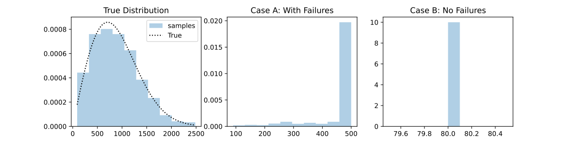
In this experiment, $500$ random numbers are generated from a Weibull distribution with $\alpha=1000$ and $\beta=2$. There are two cases of right-censored data:
- Case A: Includes failures, with a censor limit of $500$.
- Case B: No failures, with a censor limit is $80$.
Figure 1 shows the data distributions.
MLE
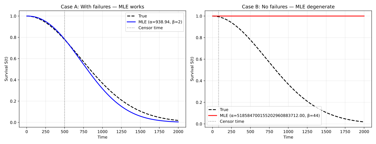
The results of the Weibull fit using MLE are shown in Figure 2. For the data with failures, the estimated parameter values are reasonably close to the true values. However, for the data without failures, the numerical optimization settles on an excessively large $\alpha$, resulting in a comp incorrect survival probability.
.
Bayesian Fit
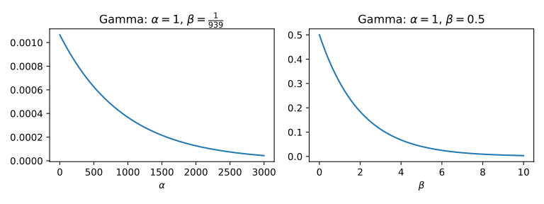
The key component of the Bayesian approach is the selection of priors. To establish them here, we assume the samples without failures (Case B) share the same intrinsic distribution as the sample with failures (Case A). Using the MLE result for Case A, we can construct the priors such that the mean of the parameter distribution aligns with the MLE result, while keeping the variance large to reflect our uncertainty. For example, we use the Gamma distributions for the priors, as shown in Figure 3.
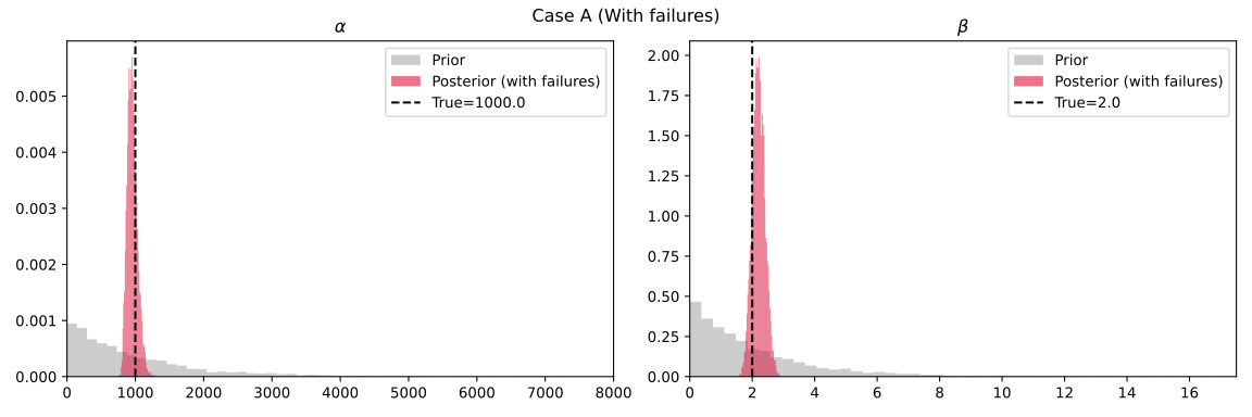
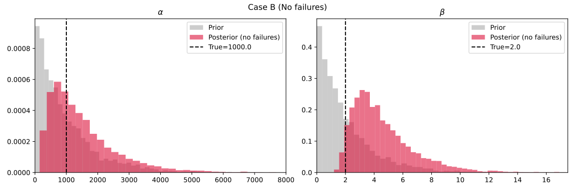
The results of the Bayesian Weibull fit using Markov chain Monte Carlo (MCMC) are shown in Figure 4 for Case A (with failures) and Figure 5 for Case B (no failures), comparing the prior, posterior, and the true values. The posterior distribution has a much wider spread when there are no failures, reflecting the lack of structural information that actual failure data typically provides.
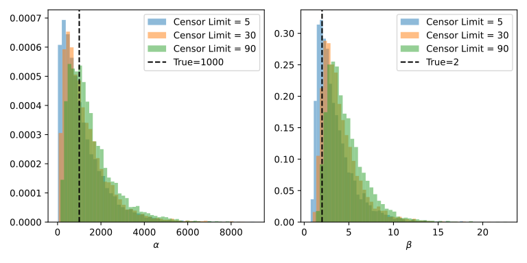
Furthermore, the posterior of the Weibull parameters in Case B (no failures) is mostly determined by the priors. In Figure 6, various censor limits are compared for Case B. While the posteriors shift slightly with the censor limit, the overall distribution remains largely the same, indicating a strong influence from the prior.
Conclusion
Fitting right-censored data without failures to a Weibull distribution can be successfully handled using a Bayesian approach. It is crucial to select reasonable priors based on domain knowledge regarding the observed data. In this study, we assume the right-censored data without failures share the same intrinsic distribution as comparable data with failures. The MLE fitting results from the data with failures were then used to construct the priors and estimate the posteriors for the failure-free data.
Appendix
Python code for Simulated Data and MLE
import numpy as np
from scipy.optimize import minimize
from scipy.stats import weibull_min, norm
import matplotlib.pyplot as plt

rng = np.random.default_rng(42)

# ---------- 1. Same simulated data as Bayesian version ----------
TRUE_ALPHA = 1000.0
TRUE_BETA  = 2.0
N = 500
CENSOR_TIME_A = 500.0
CENSOR_TIME_B = 80.0

true_times = rng.weibull(TRUE_BETA, size=N) * TRUE_ALPHA

# Case A: with failures
observed_A = np.minimum(true_times, CENSOR_TIME_A)
event_A    = (true_times <= CENSOR_TIME_A).astype(int)

# Case B: no failures
observed_B = np.full(N, CENSOR_TIME_B)
event_B    = np.zeros(N, dtype=int)

print(f"Case A: {event_A.sum()}/{N} failures")
print(f"Case B: {event_B.sum()}/{N} failures")

# ---------- 2. Negative log-likelihood ----------
def neg_loglik(params, times, events):
    """params = [log_alpha, log_beta] for unconstrained optimization."""
    log_alpha, log_beta = params
    alpha = np.exp(log_alpha)
    beta  = np.exp(log_beta)

    # log pdf and log survival
    z = (times / alpha) ** beta
    log_pdf  = np.log(beta) - np.log(alpha) + (beta - 1) * (np.log(times) - np.log(alpha)) - z
    log_surv = -z

    ll = np.sum(events * log_pdf + (1 - events) * log_surv)
    return -ll


def fit_mle(times, events, x0=None):
    if x0 is None:
        # Data-driven initialization: use mean of observed times as scale guess
        x0 = (np.log(np.mean(times)), np.log(1.5))
    res = minimize(neg_loglik, x0=x0, args=(times, events),
                   method="Nelder-Mead",
                   options={"xatol": 1e-8, "fatol": 1e-8, "maxiter": 10000})
    alpha_hat = np.exp(res.x[0])
    beta_hat  = np.exp(res.x[1])
    return alpha_hat, beta_hat, res


# ---------- 3. Fit both cases ----------
print("\n=== Case A: With failures (MLE) ===")
a_A, b_A, res_A = fit_mle(observed_A, event_A)
print(f"  alpha_hat = {a_A:.4f}  (true={TRUE_ALPHA})")
print(f"  beta_hat  = {b_A:.2f}  (true={TRUE_BETA})")


print("\n=== Case B: No failures (MLE) ===")
a_B, b_B, res_B = fit_mle(observed_B, event_B)
print(f"  alpha_hat = {a_B:.4f}")
print(f"  beta_hat  = {b_B:.2f}  <-- watch this diverge with more iterations")
print(f"  Converged? {res_B.success}, final NLL={res_B.fun:.4f}")


# ---------- 4. Demonstrate divergence of beta for no-failure case ----------
print("\n=== Demonstrating MLE divergence (no failures) ===")
print("Profile likelihood: fix beta, optimize alpha")
alpha_grid = np.array([300, 500, 1e3, 1e4, 1e5, 1e6, 1e8])
for alpha_fixed in alpha_grid:
    # minimize over alpha only
    res = minimize(lambda la: neg_loglik((la[0], np.log(alpha_fixed)), observed_B, event_B),
                   x0=[np.log(1.5)], method="Nelder-Mead")
    print(f"  alpha={alpha_fixed:.0e}  ->  NLL={res.fun:.4f}  (keeps decreasing)")

# ---------- 5. Bootstrap CI for Case B (also fails) ----------
print("\n=== Bootstrap for Case B (no failures) ===")
B = 200
boot_alphas, boot_betas = [], []
for _ in range(B):
    idx = rng.integers(0, N, N)
    try:
        a_b, b_b, _ = fit_mle(observed_B[idx], event_B[idx])
        boot_alphas.append(a_b); boot_betas.append(b_b)
    except Exception:
        pass
boot_alphas = np.array(boot_alphas); boot_betas = np.array(boot_betas)
print(f"  Bootstrap beta: median={np.median(boot_betas):.1f}, "
      f"max={boot_betas.max():.1f}  <-- unbounded")

# ---------- 6. Comparison plot ----------
fig, axes = plt.subplots(1, 2, figsize=(13, 5))
t_plot = np.linspace(1, 2000, 500)

# Case A
S_true = np.exp(-(t_plot / TRUE_ALPHA) ** TRUE_BETA)
S_mle  = np.exp(-(t_plot / a_A) ** b_A)
axes[0].plot(t_plot, S_true, "k--", lw=2, label="True")
axes[0].plot(t_plot, S_mle,  "b-",  lw=2, label=f"MLE (α={a_A:.2f}, β={b_A:.0f})")
axes[0].axvline(CENSOR_TIME_A, color="gray", ls=":", label="Censor time")
axes[0].set_title("Case A: With failures — MLE works")
axes[0].set_xlabel("Time"); axes[0].set_ylabel("Survival S(t)")
axes[0].legend(); axes[0].grid(alpha=0.3)

# Case B
S_mle_B = np.exp(-(t_plot / a_B) ** b_B)
axes[1].plot(t_plot, S_true, "k--", lw=2, label="True")
axes[1].plot(t_plot, S_mle_B, "r-", lw=2, label=f"MLE (α={a_B:.2f}, β={b_B:.0f})")
axes[1].axvline(CENSOR_TIME_B, color="gray", ls=":", label="Censor time")
axes[1].set_title("Case B: No failures — MLE degenerate")
axes[1].set_xlabel("Time"); axes[1].set_ylabel("Survival S(t)")
axes[1].legend(); axes[1].grid(alpha=0.3)

plt.tight_layout();
plt.show()
Bayesian Fit with MCMC
import numpy as np
import pymc as pm
import arviz as az
import matplotlib.pyplot as plt
import pytensor.tensor as pt

# ---------- Bayesian model ----------
def fit_weibull_censored(times, events, draws=2000, tune=2000):
    times  = np.asarray(times, dtype=float)
    events = np.asarray(events, dtype=int)

    with pm.Model() as model:
        # Weakly-informative priors (crucial for no-failure case)
        alpha = pm.Gamma("alpha", alpha=1, beta=1/939)    # mean=939
        beta  = pm.Gamma("beta",  alpha=1.0, beta=0.5) # mean=2

        # Log-likelihood: failures contribute logpdf, censored contribute logsf
        # The definition of alpha and beta is different in pyMC
        weibull = pm.Weibull.dist(alpha=beta, beta=alpha)
        logp_fail = pm.logp(weibull, times)
        # Survival function: log S(t) = -(t/alpha)^beta
        log_surv  = -(times / alpha) ** beta

        loglik = events * logp_fail + (1 - events) * log_surv
        pm.Potential("censored_likelihood", loglik.sum())

        idata = pm.sample(draws=draws, tune=tune, target_accept=0.95,
                          random_seed=42, progressbar=False)
    return idata

## Fitting Case A (with failures)
idata_A = fit_weibull_censored(observed_A, event_A)

## Fitting Case B (no failures)
idata_B = fit_weibull_censored(observed_B, event_B)

# ---------- Summaries ----------
print("\n=== Case A: With failures ===")
print(az.summary(idata_A, var_names=["alpha", "beta"], hdi_prob=0.95))

print("\n=== Case B: No failures (all censored) ===")
print(az.summary(idata_B, var_names=["alpha", "beta"], hdi_prob=0.95))