Learning Data Distribution with Planar Flow Networks
This note uses a planar flow network to learn the distribution of observed one-dimensional random values. The necessary monotonicity condition for the planar flow to be valid is derived and successfully verified through numerical experiments.
Introduction
Neural networks offer a flexible approach to learning the distribution of random variables from observed data without relying on predefined functional forms. Once trained, the learned model can generate new random samples. One effective implementation for this type of transformation is a planar flow network.
Distribution Learning
In distribution learning, a neural network acts as a transforming function that maps a known base distribution to an unknown target distribution. Specifically, the network transforms samples from a uniform distribution and compares the distribution of these transformed values to the observed data to update its parameters. After training, the network can reliably generate new samples from the target distribution by continuously feeding it uniform random samples
Monotonicity and Planar Flow
To preserve the correct order and probabilities of the data, the distribution transformation must maintain monotonicity. Planar flow is a neural network architecture designed to enforce this property. The mathematical formulation is:
\[f(z) = z + u \tanh(w z +b), \notag\]where $u$, $w$ and $b$ are parameters to be learned.
We can demonstrate that $f(z)$ can be monotonically increasing, but never monotonically decreasing. The derivative of the function is:
\[f'(z) = 1 + \frac{u w}{\cosh(w z +b)^2}. \notag\]Taking the limit as $z$ approches infinity yields:
\[\lim_{z \to \pm \infty} \frac{u w}{\cosh(w z + b)^2} = 0. \notag\]Therefore:
\[\lim_{z\to \pm \infty} f'(z) = 1 \label{eqn:df_dz_limit}\]regardless of the sign of $u w$.
Since $1\leq \cosh(w z +b)^2 < \infty$, it follows that $f’(z)\geq 1 + u w$. Consequently, if $1 + uw > 0$, then $f’(z)>0$, meaning $f(z)$ is monotonically increasing.
However, $f(z)$ cannot be monitonically decreasing because $f’(z)$ cannot be less than $0$ for all $z$ as Equation ($\ref{eqn:df_dz_limit}$) shown. This proves that $f(z)$ can only be monotonically increasing when $u w + 1 \geq 0$ and can never be monotonically decreasing.
To consistently satisty the requirement $u w + 1 > 0$, the parameters $u$ and $w$ must be constrained. One effective method is to introduce an intermediate parameter $\hat{u}$ as a function of $u$ and $w$, replacing $u$ such that $\hat{u} w +1 >0$ for any $u$ and $w$.
Let:
\[m = \log(1 + \exp(u w)) -1. \notag\]Here, $m > -1$ for all $u$ and $w$.
We then define:
\[\hat{u} = u + (m - wu) \frac{w}{\mid w\mid^2}. \notag\]We can confirm that the constraint holds:
\[\hat{u} w +1 = uw + m - uw +1 = m +1 > 0. \notag\]Planar Flow Network
The planar flow neurla netowrk and the overall distribution learning process reply on mapping uniform inputs to observed data (Figure 1).
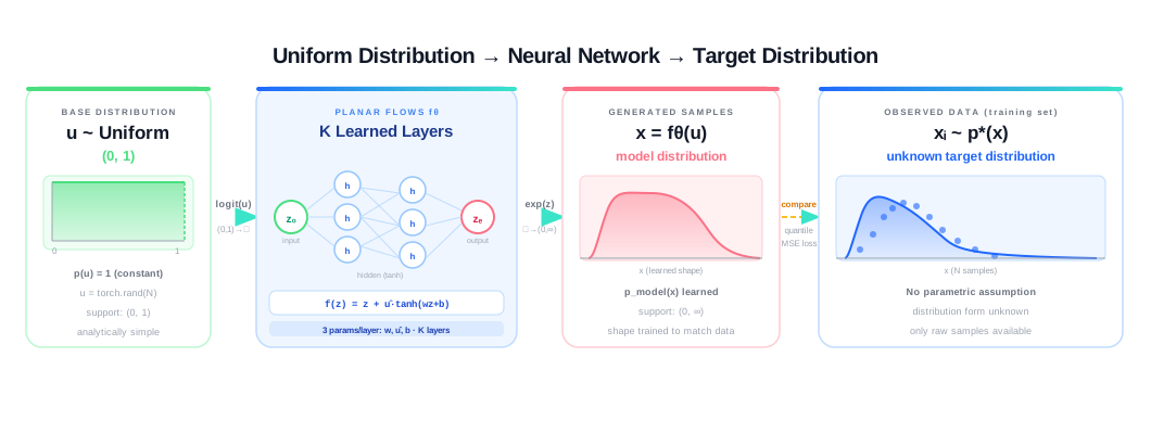
The support of the uniform distribution is $(0,1)$. Samples from this distribution are transformed to a support of $(-\infty, \infty)$ using the logit function before being passed into the planar flow network. The netowrk itself consists of multiple planar flow layers. The final output has a support of $(-\infty, \infty)$, which can be transformed to match the support of the target distriution. For instance, if the target distribution’s support is $(0, \infty)$, an expoential function is applied to the network’s output.
Results
The planar flow network is trained to learn the distribution of $1500$ random samples drawn from a Weibull distribution. The Python implementation is provided in the Appendix.
Quantile loss is used to match the quantile functions of the model and the data. The planar flow model acts as the quantile function (or the inverse CDF) of the learned distribution; by definition of the Proabability Integral Transform, any function that maps uniform input into samples from a specific distribution is that distribution’s inverse CDF. The quantile function of observed data is numrically calculated using the torch.quantile function.
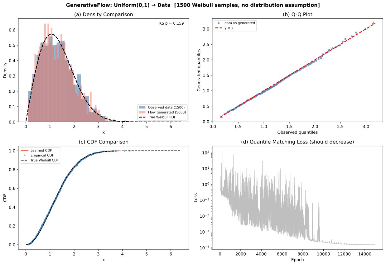
In the numrical experiments, the network consistes of $16$ planar flow layers. As shown in Figure 2, excellent agreement between the observed data and the samples generated by the trained model is demonstrated across histogram, Q-Q plots and CDF plots. Furthermore, Kolmogorov-Smirnov (KS) tests confirm that the model-generated samples are statististically consistent with both the observed empirical data and the theoretical Weibull distribution.
Generated 1500 valid samples
KS test vs true Weibull: stat=0.0289, p=0.1590
(p > 0.05 means generated samples are consistent with Weibull)
KS test vs observed data: stat=0.0260, p=0.6913
(p > 0.05 means generated samples are consistent with observed data)
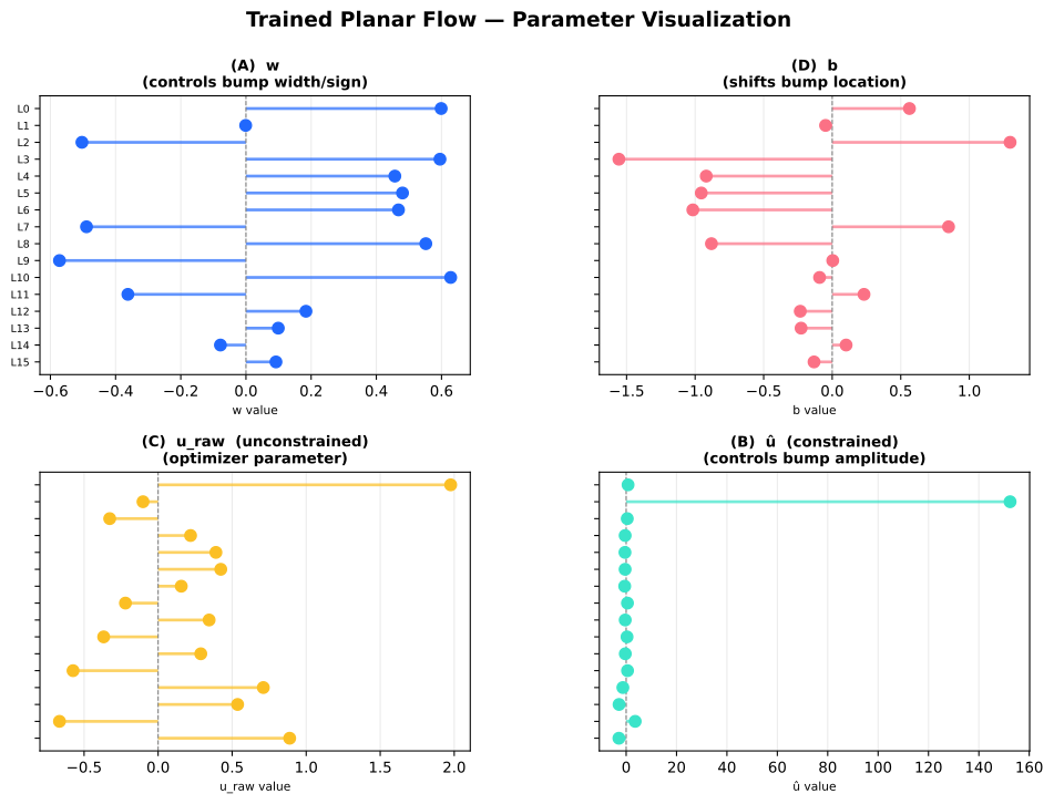
The values of the parameters of the planar flow network at each layer are shown in Figure 3.
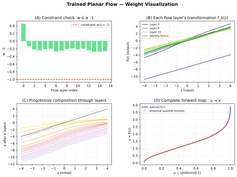
The monotonicity constraint $w\hat{u} \geq -1$ is statisfied across all plananr flow layers. Progressive composition through the layers confirms that the plananr flow transform $f(z)$ maintains proper structural behavior from input to output.
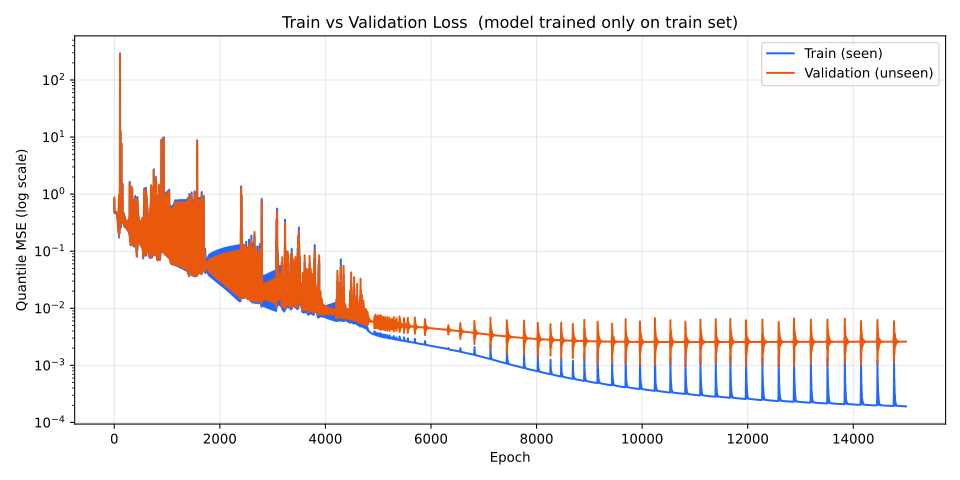
Finally, overfitting is evaluated by partitioning the $2000$ observed data points into an $80\%$ training set and a $20\%$ validattion set. Up to epoch $5000$, both training and validation losses decrease concurrently. After Epoch $5000$, the validation loss plateaus while the trainling loss continues to decease. This indicates that stopping the training around epoch $5000$ prevents the model from overfitting.
Conclusion
By mapping uniform noise through constrained, monotonically increasing planar flow layers, the model effectively learns and replicates the underlying distribution of observed data without relying on predefined parametric equations. The experimental application on Weibull-distributed samples validates this approach, showing strong statistical alignment between the generated values and the true distribution. Ultimately, monitoring the validation loss to implement early stopping ensures that the network retains generalizability while fully capturing the target distribution’s characteristics.
Appendix
Python code of Planar Flow Network
The Python code of the planar flow netowrk and training of the network to learn the distribuiton from samples from a Weibull distribtuion. The code was generated with the help of Claude Opus 4.7 model.
import torch
import torch.nn as nn
import torch.optim as optim
import numpy as np
import matplotlib.pyplot as plt
from scipy.stats import weibull_min, kstest, ks_2samp

torch.manual_seed(42)
np.random.seed(42)

# ──────────────────────────────────────────────
# 0. Generate observed data (model never sees
#    the Weibull parameters — only the numbers)
# ──────────────────────────────────────────────
WEIBULL_K, WEIBULL_LAM = 2.0, 1.5
N_DATA = 1500

data_np = weibull_min.rvs(c=WEIBULL_K, scale=WEIBULL_LAM, size=N_DATA)
data_np_sorted = np.sort(data_np)
data = torch.tensor(data_np, dtype=torch.float32)
print(f"Data: min={data_np.min():.3f} max={data_np.max():.3f} "
      f"mean={data_np.mean():.3f} std={data_np.std():.3f}")

EPS = 1e-6


# ──────────────────────────────────────────────
# 1. Single Planar Flow layer
#    f(z) = z + u_hat * tanh(w*z + b)
# ──────────────────────────────────────────────
class PlanarFlow(nn.Module):
    def __init__(self):
        super().__init__()
        self.w     = nn.Parameter(torch.randn(1) * 0.1)
        self.u_raw = nn.Parameter(torch.randn(1) * 0.1)
        self.b     = nn.Parameter(torch.zeros(1))

    def get_u_hat(self):
        """Enforce w * u_hat >= -1 for invertibility."""
        wu  = self.w * self.u_raw
        m   = torch.log1p(torch.exp(wu)) - 1.0   # softplus - 1
        return self.u_raw + (m - wu) * self.w / (self.w**2 + EPS)

    def forward(self, z):
        """
        z    : (N,) or (N,1)
        out  : same shape as z
        """
        u_hat = self.get_u_hat()
        h     = torch.tanh(self.w * z + self.b)
        return z + u_hat * h


# ──────────────────────────────────────────────
# 2. Full generative model
#
#  FORWARD (generation — Uniform → Data):
#    u  ~  Uniform(0,1)              support: (0,1)
#    z0 =  logit(u)                  support: R
#    zK =  PlanarFlow^K(z0)          support: R
#    x  =  exp(zK)                   support: (0,inf)
#
#  This is a PURELY FORWARD model — no inverse needed for training.
#  Training uses quantile matching loss (see Section 4).
# ──────────────────────────────────────────────
class GenerativeFlow(nn.Module):
    def __init__(self, n_flows=16):
        super().__init__()
        self.flows = nn.ModuleList([PlanarFlow() for _ in range(n_flows)])

    def forward(self, u):
        """
        u : (N,)  uniform samples in (0,1)
        x : (N,)  generated samples in (0,inf)
        """
        u = u.clamp(EPS, 1 - EPS)

        # logit: (0,1) -> R
        z = torch.log(u) - torch.log(1.0 - u)

        # planar flows: R -> R
        for flow in self.flows:
            z = flow(z)

        # exp: R -> (0, inf)
        x = torch.exp(z.clamp(-12, 12))
        return x


# ──────────────────────────────────────────────
# 3. Loss function: Quantile Matching (Cramer loss)
#
#  Key insight: if we feed SORTED uniform inputs
#  u_(1) < u_(2) < ... < u_(N)  into the flow,
#  the outputs x_(i) = f(u_(i)) are also sorted
#  (flow is monotone). These are the model's
#  empirical quantiles.
#
#  We match them to the SORTED observed data:
#    Loss = (1/N) * sum_i  (x_(i) - data_(i))^2
#
#  This is the squared Cramer / energy distance —
#  it is minimized when the two distributions match.
#  Gradients flow cleanly through the forward pass.
#
#  Why does this work?
#    - x_(i) = F_model^{-1}(u_(i)) = model quantile
#    - data_(i) = empirical quantile of observed data
#    - Minimizing MSE between quantiles = minimizing
#      the Cramer distance between distributions
# ──────────────────────────────────────────────
# def quantile_loss(model, data_sorted_tensor, n_samples=1000):
#     """
#     data_sorted_tensor : (N,) sorted observed data
#     n_samples          : number of uniform quantile points
#     """
#     N = len(data_sorted_tensor)

#     # Evenly-spaced quantile levels — same for both model and data
#     # Use (i+0.5)/n_samples to avoid 0 and 1
#     levels = torch.linspace(0, 1, n_samples + 2)[1:-1]   # (n_samples,)

#     # Model quantiles: forward pass through flow
#     x_model = model(levels)                               # (n_samples,)

#     # Data quantiles: interpolate from sorted data
#     # levels are in (0,1), map to index in [0, N-1]
#     idx_float = levels * (N - 1)
#     idx_lo    = idx_float.long().clamp(0, N - 2)
#     idx_hi    = (idx_lo + 1).clamp(0, N - 1)
#     frac      = (idx_float - idx_lo.float()).clamp(0, 1)
#     x_data    = (data_sorted_tensor[idx_lo] * (1 - frac)
#                  + data_sorted_tensor[idx_hi] * frac)     # (n_samples,)

#     # MSE between quantiles
#     loss = ((x_model - x_data) ** 2).mean()
#     return loss

# simpler loss function
def quantile_loss(model, data_tensor, n_samples=1000):
    """
    data_tensor : (N,)  observed data (does NOT need to be pre-sorted)
    n_samples   : number of quantile levels to match
    """
    # Evenly spaced quantile levels in (0, 1) — exclude endpoints
    levels = torch.linspace(0, 1, n_samples + 2)[1:-1]   # (n_samples,)

    # Model quantiles: forward pass
    x_model = model(levels)                               # (n_samples,)

    # Data quantiles: direct torch.quantile call
    x_data  = torch.quantile(data_tensor, levels)         # (n_samples,)

    return ((x_model - x_data) ** 2).mean()


# ──────────────────────────────────────────────
# 4. Verify monotonicity (planar flow in 1D
#    IS monotone when u_hat satisfies the constraint)
# ──────────────────────────────────────────────
def check_monotone(model):
    with torch.no_grad():
        u_test = torch.linspace(0.01, 0.99, 200)
        x_test = model(u_test)
        diffs  = x_test[1:] - x_test[:-1]
        n_violations = (diffs <= 0).sum().item()
    print(f"  Monotonicity check: {n_violations} violations "
          f"(should be 0 for valid training)")
    return n_violations == 0


# ──────────────────────────────────────────────
# 5. Training loop
# ──────────────────────────────────────────────
def train(model, data_np, n_epochs=3000, lr=1e-3, n_samples=1000):
    # Pre-sort data once
    data_sorted = torch.tensor(np.sort(data_np), dtype=torch.float32)

    optimizer = optim.Adam(model.parameters(), lr=lr)
    scheduler = optim.lr_scheduler.CosineAnnealingLR(
                    optimizer, T_max=n_epochs, eta_min=1e-5)
    losses = []

    for epoch in range(n_epochs):
        model.train()

        loss = quantile_loss(model, data_sorted, n_samples=n_samples)

        if torch.isnan(loss) or torch.isinf(loss):
            print(f"  [warn] NaN/Inf loss at epoch {epoch+1}, stopping")
            break

        optimizer.zero_grad()
        loss.backward()
        nn.utils.clip_grad_norm_(model.parameters(), max_norm=2.0)
        optimizer.step()
        scheduler.step()

        losses.append(loss.item())

        if (epoch + 1) % 500 == 0:
            print(f"  Epoch {epoch+1:5d} | Loss: {loss.item():.6f}")

    return losses


# ──────────────────────────────────────────────
# 6. Run
# ──────────────────────────────────────────────
model = GenerativeFlow(n_flows=16)

print("\nChecking monotonicity before training:")
check_monotone(model)

print("\nTraining...")
losses = train(model, data_np, n_epochs=15000, lr=2e-3, n_samples=1000)

print("\nChecking monotonicity after training:")
check_monotone(model)

# ── Generate samples ──────────────────────────
model.eval()
with torch.no_grad():
    u_gen   = torch.rand(1500).clamp(EPS, 1 - EPS)
    x_gen   = model(u_gen).numpy()
    x_clean = x_gen[(x_gen > 0) & (x_gen < data_np.max() * 4)]

print(f"\nGenerated {len(x_clean)}/5000 valid samples")

# ── KS test: generated distribution vs. Weibull ──
ks_s, ks_p = kstest(x_clean,
                     weibull_min(c=WEIBULL_K, scale=WEIBULL_LAM).cdf)
print(f"KS test vs true Weibull: stat={ks_s:.4f}, p={ks_p:.4f}")
print("(p > 0.05 means generated samples are consistent with Weibull)")

# ── KS test: generated distribution vs. training data ──
ks2_s, ks2_p = ks_2samp(x_clean, data_np)
print(f"KS test vs observed data: stat={ks2_s:.4f}, p={ks2_p:.4f}")
print("(p > 0.05 means generated samples are consistent with observed data)")

# ──────────────────────────────────────────────
# 7. Plots
# ──────────────────────────────────────────────
x_plot   = np.linspace(0.01, data_np.max() * 1.5, 400)
true_pdf = weibull_min.pdf(x_plot, c=WEIBULL_K, scale=WEIBULL_LAM)

fig, axes = plt.subplots(2, 2, figsize=(13, 9))
fig.suptitle(
    f"GenerativeFlow: Uniform(0,1) → Data  "
    f"[{N_DATA} Weibull samples, no distribution assumption]",
    fontsize=12, fontweight='bold'
)

# (a) Density
ax = axes[0, 0]
ax.hist(data_np, bins=25, density=True, alpha=0.6,
        color='steelblue', label=f'Observed data ({N_DATA})')
ax.hist(x_clean, bins=60, density=True, alpha=0.45,
        color='tomato', label='Flow generated (5000)')
ax.plot(x_plot, true_pdf, 'k--', lw=2, label='True Weibull PDF')
ax.set_title('(a) Density Comparison')
ax.set_xlabel('x');  ax.set_ylabel('Density')
ax.legend(fontsize=8)
ax.text(0.97, 0.97, f'KS p = {ks_p:.3f}',
        transform=ax.transAxes, ha='right', va='top', fontsize=9,
        color='k' if ks_p > 0.05 else 'red')

# (b) Quantile-quantile: model vs data
ax = axes[0, 1]
q  = np.linspace(1, 99, 99)
ax.plot(np.percentile(data_np, q), np.percentile(x_clean, q),
        'o', ms=4, alpha=0.7, color='steelblue', label='data vs generated')
lo = min(np.percentile(data_np, 1), np.percentile(x_clean, 1))
hi = max(np.percentile(data_np, 99), np.percentile(x_clean, 99))
ax.plot([lo, hi], [lo, hi], 'r--', lw=2, label='y = x')
ax.set_title('(b) Q-Q Plot')
ax.set_xlabel('Observed quantiles')
ax.set_ylabel('Generated quantiles')
ax.legend(fontsize=8)

# (c) Learned CDF vs empirical CDF
ax = axes[1, 0]
with torch.no_grad():
    u_grid = torch.linspace(0.001, 0.999, 500)
    x_grid = model(u_grid).numpy()
ax.plot(x_grid, u_grid.numpy(),
        color='tomato', lw=2, label='Learned CDF')
x_emp_sorted = np.sort(data_np)
p_emp        = np.arange(1, N_DATA + 1) / (N_DATA + 1)
ax.plot(x_emp_sorted, p_emp,
        'o', ms=3, alpha=0.5, color='steelblue', label='Empirical CDF')
ax.plot(x_plot, weibull_min.cdf(x_plot, c=WEIBULL_K, scale=WEIBULL_LAM),
        'k--', lw=1.5, label='True Weibull CDF')
ax.set_title('(c) CDF Comparison')
ax.set_xlabel('x');  ax.set_ylabel('CDF')
ax.legend(fontsize=8)

# (d) Training loss
ax = axes[1, 1]
ax.plot(losses, alpha=0.25, color='k', lw=1, label='raw')
ax.set_title('(d) Quantile Matching Loss (should decrease)')
ax.set_xlabel('Epoch');  ax.set_ylabel('Loss')
ax.set_yscale('log')
Referneces
Variational Inference with Normalizing Flows, Rezende & Mohamed, 2015
Probability Integral Transform, Wikipedia.