Quantifying Uncertainty in Reliability Comparisons: A Simulation Study of the Log-Rank Test and Cox Model
When ranking the reliability of two groups by comparing survival data, uncertainty arising from finite sample sizes and data censoring can lead to incorrect conclusions. In this note, we use numerical simulations to quantify how these factors influence the probability of “incorrect ranking”—specifically, finding a difference when none exists (Type I error). Our findings demonstrate that statistical significance tests, such as the log-rank test, reliably control this probability regardless of sample size or censoring levels.
Simulation Framework
To investigate these effects, we simulate two groups of time-to-failure data randomly drawn from the exact same underlying distribution. Since the groups are identical, any observed difference is purely due to stochastic noise.
Weibull Distribution
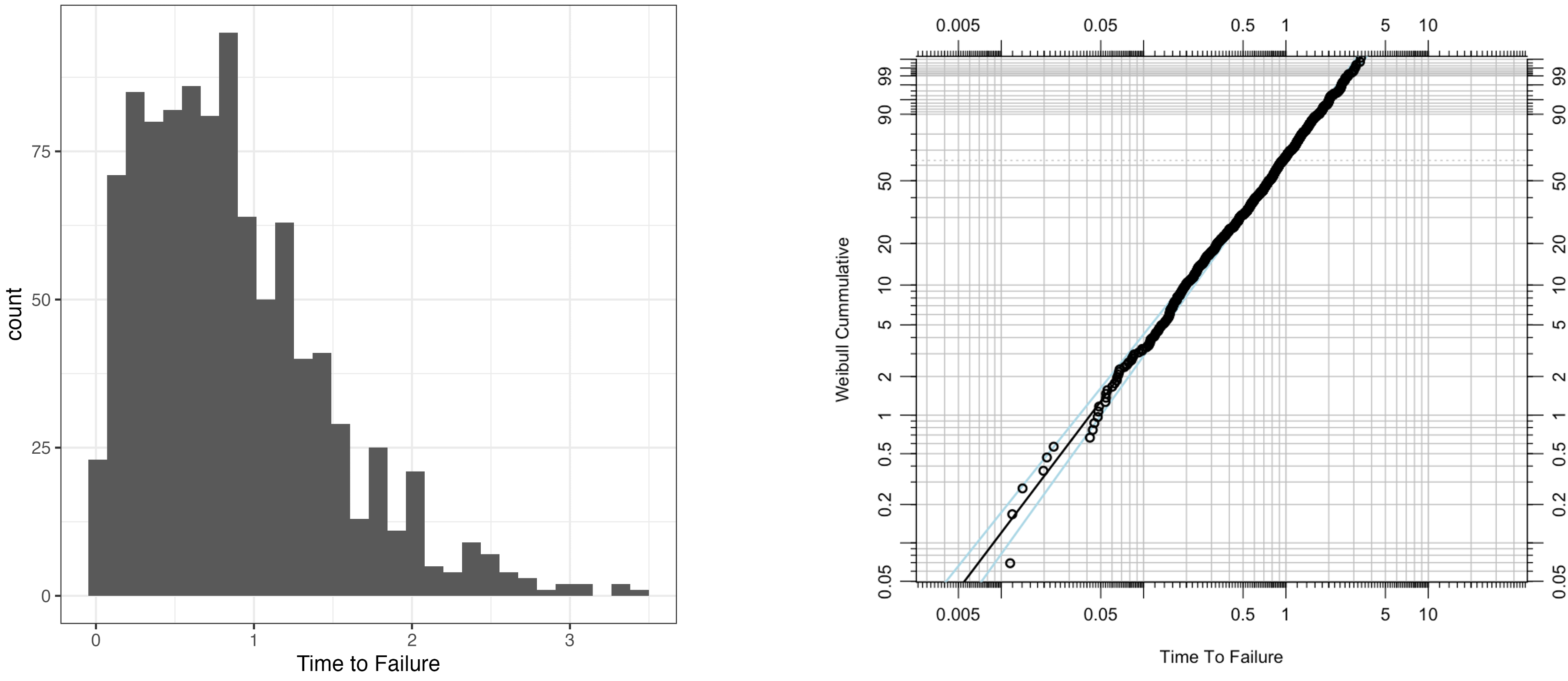
We assume that the time-to-failure follows a Weibull distribution. The probability density function (PDF) with scale parameter $\alpha$ and the shape parameter $\beta$ is defined as:
\[f(t; \alpha, \beta)=\frac{\beta e^{-\left(\frac{t}{\alpha }\right)^{\beta }} \left(\frac{t}{\alpha }\right)^{\beta -1}}{\alpha }. \notag\]The complimentary cummulative distribution function (CCDF), or survival function, is
\[\text{CCDF}(t) = e^{-\left(\frac{t}{\alpha}\right)^\beta}. \notag\]Figure 1 illustrates $1000$ samples drawn from a Weibull distribution with $\alpha=1$ and $\beta = 1.5$.
Comparison of Two Groups: Survival Curves
We generate 1000 pairs of samples (size $n=50$) from the same distribution. Even with identical parameters, sampling variation creates apparent differences in survival curves.
library(tidyverse)
library(survival)
library(ggsurvfit)

set.seed(1234)
ss <- 50 #sample size
nboot <- 1000 #number of bootstraps
beta <- 1.5 # weibull shape
scale <- 1 # weibull scale

data <-
data.frame(time_to_event = rweibull(n = 2*ss*nboot, shape = beta, scale = scale),
                        status =1) |>
    mutate(bootsample = (row_number() -1 ) %/% (2*ss),
           group = row_number() %% 2)
As whon in Figure 2, some iterations show significant visual divergence. The p-value from the log-rank test is used to determine if these observed differences are statistically significant.

The Effect of Sample Size
We can quantify the apparent difference between groups using the hazard ratio (HR) from a Cox Proportional Hazards model and the p-value of the log-rank test. We simulated various sample sizes ($n=10,50,100,500$) to observe the distribution of hazard ratio and p-values.
library(tidyverse)
library(survival)

# --- Simulation Function ---
run_hr_sim <- function(ss, nboot = 1000, beta = 1.5, scale = 1) {
  # ss: sample size
  # nboot: number of bootstraps
  # beta: shape of Weibull distribution
  # scale: scale of Weibull distrbution
  set.seed(1234)

  # Total observations needed
  n_total <- 2 * ss * nboot

  # Generate data efficiently
  data_sim <- data.frame(
    t_fail   = rweibull(n_total, shape = shape, scale = scale),
    t_censor = 10^7, # Effectively no censoring
    bootsample = rep(1:nboot, each = 2 * ss),
    group      = rep(c(0, 1), times = ss * nboot)
  ) |>
    mutate(
      time   = pmin(t_fail, t_censor),
      status = as.numeric(t_fail < t_censor) # true event or censored
    )

  # Harzard ratio and log-rank test p-value for each bootstrap sample
  data_sim |>
    group_by(bootsample) |>
    group_modify(~ {
      # Fit models
      fit_cox  <- coxph(Surv(time, status) ~ group, data = .x)
      fit_diff <- survdiff(Surv(time, status) ~ group, data = .x)

      # Extract stats
      hr_val <- exp(coef(fit_cox))
      tibble(
        # Standardizing HR to be >= 1 for variation analysis
        hr   = if_else(hr_val > 1, hr_val, 1 / hr_val),
        pval = fit_diff$pvalue,
        ss   = ss
      )
    }) |>
    ungroup()
}

# --- Execution ---
sample_sizes <- c(10, 50, 100, 500)

hr_results <- map_dfr(sample_sizes, run_hr_sim)
- Hazard ratio (Figure 3): Smaller sample sizes lead to much larger variations in the estimated hazard ratio. With $n=10$, a high hazard ratio may appear purely by chance.
- P-value (Figure 4): Interestingly, the distribution of p-value remains uniform (a 1:1 diagonal line on the CDF) regardless of sample size.
This confirms that the log-rank test consistently controls the false positive rate. If we set $\alpha=0.05$, we will incorrectly conclude the groups are different only $5\%$ of the time, whether $n$ is $10$ or $500$.


The Effect of Censoring
Censoring occurs when a faikure is not observed within the study periosd. We simulated this by applying a cut-off threshold to the lifetime data.
-
Hazard ratio (Figure 5): Increased censoring increases the variance of the hazard ratio.
-
P-value (Figure 6): The p-value distribution remains robust and insenitive to the censoring proportion.


Conclusion
Uncertainty in reliability comaprisons stems from finite sampling and data censoring. This study higlights two distinct behaviors:
- The hazard ratio is highly sensitive. heavy censoring can produce misleadingly larger hazard ratio values.
- The log-rank p-value is remarkably robust, Its distribution remains uniform under the null hypothesis, ensuring that the false positive rate is controlled by rhechosen significnace threshold.
This result shows that while hazard ratio is noisy in small trials, the log-rank test remains a reliable metric for statistical validity.