Variational Autoencoder for CelebA Image Analysis
In this note, we implement a variational autoencoder (VAE) using the neural network framework in Wolfram Language and train it on the CelebFaces Attributes (CelebA) dataset. New images can be generated by sampling from the learned latent space. We explore how the VAE captures and manipulates image features, particularly the concept of attractiveness.
Model
VAEs are a type of deep learning model that can learn latent representations of data. As illustrated in Figure 1, an encoder network takes an input image $x$ is and compresses it into a latent variable $z$. This latent space captures the essence of the image. A decoder network takes the latent variable $z$ and reconstructing an image $x’$ that resembles the original input $x$.The decoder represents the conditional probability $p(x\vert z)$ and the encoder presents the probability $q(z\vert x)$, which approximates the distribution of $z$ in latent space. In this implementation, the distribution of $z$ is a multivariate Gaussian.

The encoder and decoder are constructed with multiple convolutional layers and transposed convolution layers, respectively. The encoder uses convolutional layers to compress the image’s information progressively. The decoder performs the opposite task. It takes the latent variable, essentially a compressed representation of the image, and employs transposed convolutional layers to progressively upscale and rebuild the image.
Dataset
The CelebFaces Attributes (CelebA) Dataset provides $202599$ celebrity images, each labeled with $40$ facial attributes, including attractiveness.
Wolfram Language Implementation
The deep network VAE is implemented in Wolfram Language. The network structure is adopted from Generative Deep Learning by David Foster.
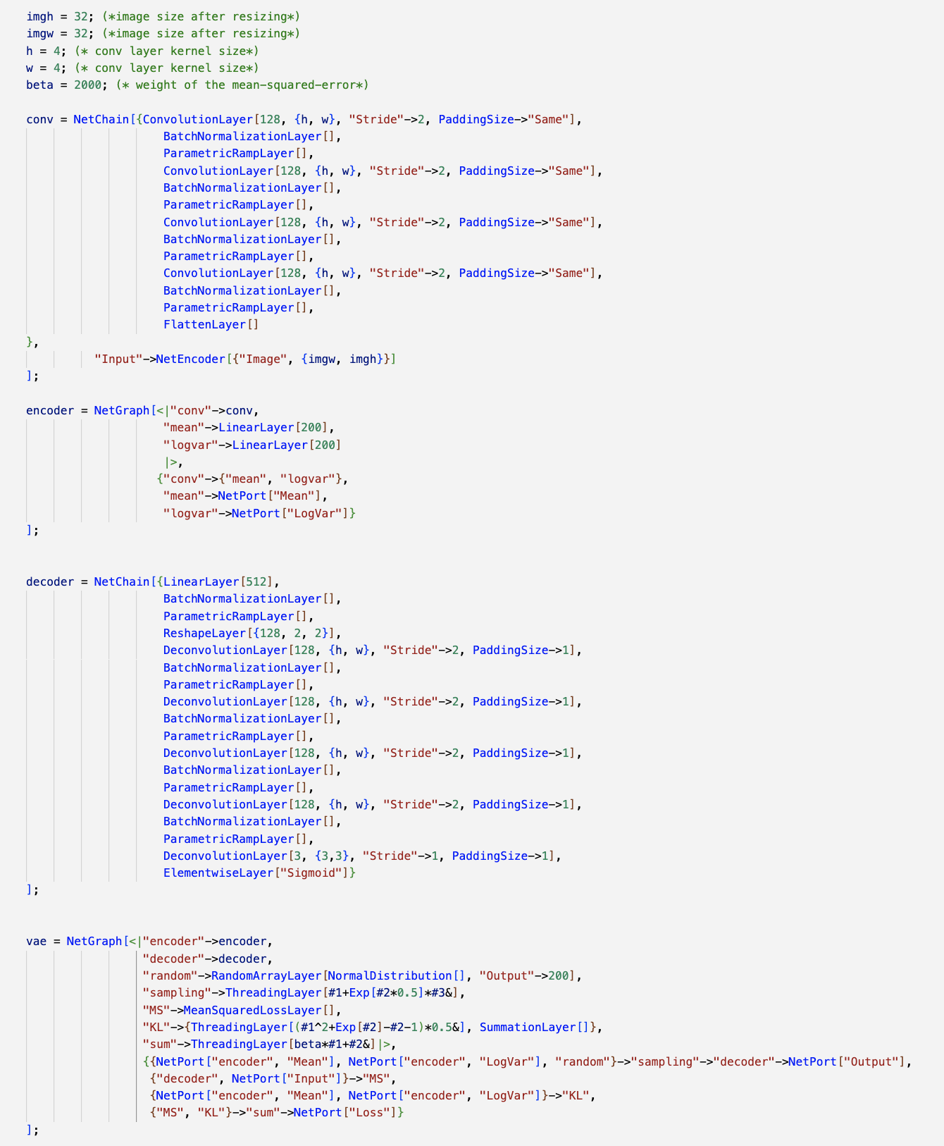
In this implementation, we use the VAE structure, which consists of an encoder and a decoder (Figure 2). The encoder has four convolutional layers; its structure is shown in Figures 3 and 4. The output of the encoder is the mean and logarithm of the multivariate Gaussian distribution with a dimension of $200$. We assume that the covariance matrix of the Gaussian distribution is diagonal, which means the logarithm of the variance is a one-dimensional array. On the other hand, the decoder has five transposed convolutional layers (or Deconvolution layers in Wolfram Language), as shown in Figure 5. The decoder takes random samples from the multivariate Gaussian distribution and produces the decoded images as output.


The loss function used in this model consists of two parts. Firstly, it involves calculating the mean squared error between the input image and the decoded image from the decoder. Secondly, it includes computing the Kullback-Leibler (KL) divergence between the multivariate Gaussian distribution generated by the encoder and a multivariate normal distribution. The KL divergence is calculated using the below formula:
\[D_{KL} = \frac{1}{2}\sum_i \left(\mu_i^2+\exp(\log\sigma_i^2)-\log\sigma_i-1\right). \notag\]Here, $\mu_i$ and $\sigma_i^2$ represent the mean and variance of the multivariate Gaussian distribution that is generated by the encoder.
The original images, with size $178\times218$, were reduced to $32\times32$ for faster computation.
Training
The VAE is trained on all 202599 images in the CelebA dataset using a GPU. It undergoes ten rounds of training. The loss plot in Figure 6 shows that ten rounds of training are sufficient.
files = File/@FileNames[All,"data/archive/img_align_celeba/img_align_celeba"]

result = NetTrain[vae, files, All, LossFunction->"Loss", BatchSize->500,  TargetDevice->{"GPU", All}, MaxTrainingRounds->10];

Result
Image Generation
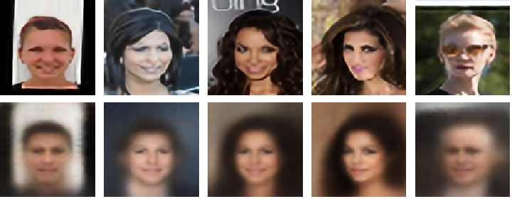
In Figure 7, the input images are in the top row, which were fed into the trained VAE model. The corresponding output images are in the bottom row. These images were upscaled from $32\times 32$ pixel size to $96\times 96$ using the Very Deep Convolutional Networks, which is an architecture inspired by VGG. The trained network from Wolfram Neural Net Repository was used to achieve this.
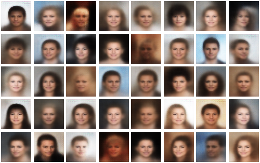
Once the VAE was trained, it became capable of generating entirely new, realistic-looking images. The VAE achieves this by sampling random points from the learned latent space and feeding them to the decoder. The decoder, having learned the relationships between latent variables and image features, can produce novel images that reside within the distribution of the training data. Figure 8 shows $40$ random images generated this way.
Visualizing Convolutional Layers
To understand how the VAE processes images, we examine the outputs of each convolutional layer in the encoder and decoder. For this purpose, we input a single image (Figure 9) into the VAE, and then observe and display the resulting outputs of the convolutional layers.

Convulaitonal Layers in the Encoder
Figures 10-13 shows the encoder progressively extracts higher-level features from the input image during the encoding phase.


Convolution Layers in the Decoder
Figures 14-18 show the decoder gradually builds up the image from the latent representation, reintroducing more details layer by layer.


Morphing Attractiveness in Latent Space
The encoder converts training images into a a 200-dimensional multivariate normal distribution within the latent space, where each image can be represented by the mean, a 200-dimensional vector in the latent space. To visually explore the image distribution in the latent space, we use the UMAP dimesnional reduction method, which condenses the 200-dimensional vectors into a 2-dimensional space.
Addtionally, each image receives a label indicating attractiveness ($\mathrm{attractive}=1$) or unattractiveness ($\mathrm{attractive}=-1$). Figure 19 shows distinct distribions for attractive and unattractive images in the latent space.

Let’s define $\Delta$ as the difference between the means of attrative and unattractive images in the latent space. Altering an image involves adding multiples of $\Delta$ to its latent space representation:
\[z' = z + n\Delta, \notag\]where $z$ is the latent space representation of an image, $n$ is a real multiplier, and $z’$ denotes the modified representation.
Figure 20 illustrate the transition of four images transitioning from more attractive to less attractive. This transiiton suggests that more attractive individuals tend to have longer hair instead of being bald, exhibit plumber features, and possess more feminite characteristics.

Conclusion
The variational autoencoder efficiently converts images into probability distributions within latent space, capturing not just objective features like hair length but also subjective attributes such as attractiveness. Implementing this deep network is straightforward using the Neural Network Framework available in the Wolfram Language.
References
Foster, David (2023). Generative Deep Learning: Teaching Machines To Paint, Write, Compose, and Play (2nd ed.). O’Reilly Media, Inc.
CelebFaces Attributes (CelebA) Dataset
Very Deep Net for Super-Resolution
UMAP:Uniform Manifold Approximation and Projection for Dimension Reduction