Numerical Investigation of the Lorenz System
We solve the ordinary differential equations of the Lorenz system to generate time series for future prediction with various models, including XGBoost and deep neural networks. Furthermore, we numerically compute the Lyapunov exponents of the Lorenz system to gain insights into its chaotic behavior.
Dynamics of the Lorenz System
The Lorenz system is described by a set of ordinary differential equations:
\[\begin{align} \frac{dx}{dt} &= \sigma (y-x) \\ \frac{dy}{dt} &= x (\rho - z) -y\\ \frac{dz}{dt} &= x y - \beta z \end{align} \label{eqn:lorenz}\]where $\sigma$, $\rho$, and $\beta$ are some constants.
The solution to the Lorenz System is obtained by solving the initial value problem, demonstrated through the Python code snippet below:
from scipy.integrate import solve_ivp

def lorenz(t, xyz, σ, ρ, β):
    x, y, z = xyz
    x_dot = σ*(y - x)
    y_dot = x*(ρ - z) - y
    z_dot = x*y - β*z
    return (x_dot, y_dot, z_dot)

σ = 10
ρ = 28
β = 8/3
t = np.linspace(0, 100, 10000)
t_span = (0, 100)
sol = solve_ivp(lorenz, t_span, y0=(1,1,1), t_eval=t, args=(σ, ρ, β))
Figure 1 visually represents the trajectory of the Lorenz system with $\sigma=10$, $\rho=28$, and $\beta=8/3$, with the red dot marking the initial position.

Analyzing Chaos with Lyapunov Exponents
The Lorenz System exhibits chaotic behavior, as evidenced by the strange attractor in Figure 1. To quantify this chaos, we turn to Lyapunov exponents, which measure the rate of separation of infinitesimally close trajectories.
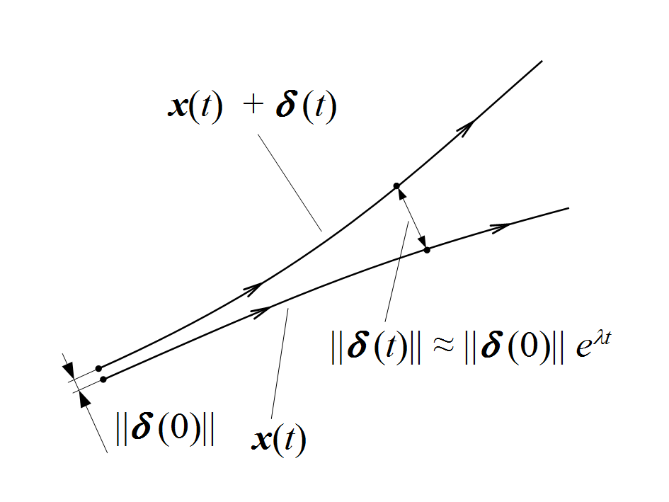
Lyapunov exponents are used to understand how closely aligned trajectories in dynamical systems, like the Lorenz system, drift apart over time. Each system has its own set of Lyapunov exponents, with the maximal one influencing the system’s behavior the most. Figure 2 illustrates this: initially close trajectories at $t=0$ separate exponentially as time progresses:
\[\vert \delta(t)\vert \approx \vert \delta(0)\vert e^{\lambda t} , \notag\]where $\lambda$ is the maximal Lyapunov exponent.
We estimate the maximal Lyapunov exponent by calculating the separation between initally close trajectories as a function of time. The results are shown in Figures 3 and 4.
δ0 = 1e-10 #initial seperation
sol = solve_ivp(lorenz, t_span, y0=(1,1,1), t_eval=t, args=(σ, ρ, β))
sol1 = solve_ivp(lorenz, t_span, y0=(1,1,1+δ0), t_eval=t, args=(σ, ρ, β))

d = (sol.y - sol1.y) # seperation
d = np.sqrt((d**2).sum(axis=0)) #seperation
Figure 3 illustrates the separation between initially close trajectories, showcasing a time range with exponential growth. The growth rate is determined through curve fitting.

Similarly, Figure 4 breaks sown the separation in $x$, $y$, and $z$ over time, highlighting exponential growth for each dimension.

Figures 5 and 6 present the sepration between two initally close trajactories for different values of $\sigma$, $\rho$, and $\beta$. The corresponding maximal Lyapunov expoenentsa re tabulated and compared with results from Viswanath (1998) .


The maximal Lyapunov exponent of the Lorenz system for there different choices of $\sigma$, $\rho$, and $\beta$ is summarized the the table below. A comparison between Viswanath’s theoretical values and our numerical results indicates a reasonally good agreement.
| $\sigma$ | $\rho$ | $\beta$ | Maximal Lyapunov Exponent $\lambda$ | Numerical Result |
|---|---|---|---|---|
| 10 | 28 | 8/3 | 0.90566 | 0.88 |
| 16 | 45.92 | 4 | 1.50255 | 1.42 |
| 16 | 40 | 4 | 1.37446 | 1.11 |
References
Viswanath, Divakar. Lyapunov exponents from random Fibonacci sequences to the Lorenz equations. Doctoral dissertation. Cornell University, 1998.