Student's t Mixture Model with PyMC
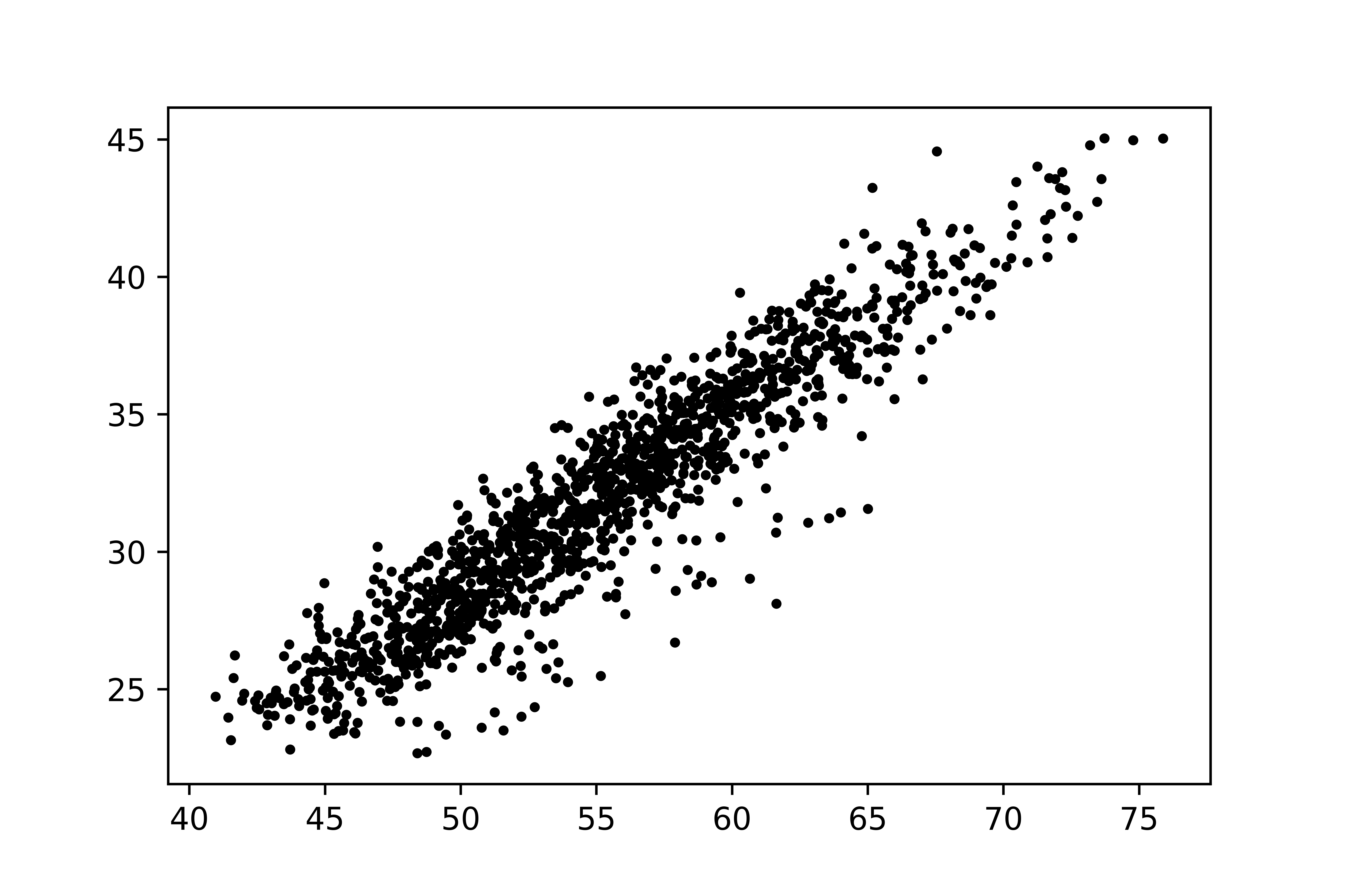
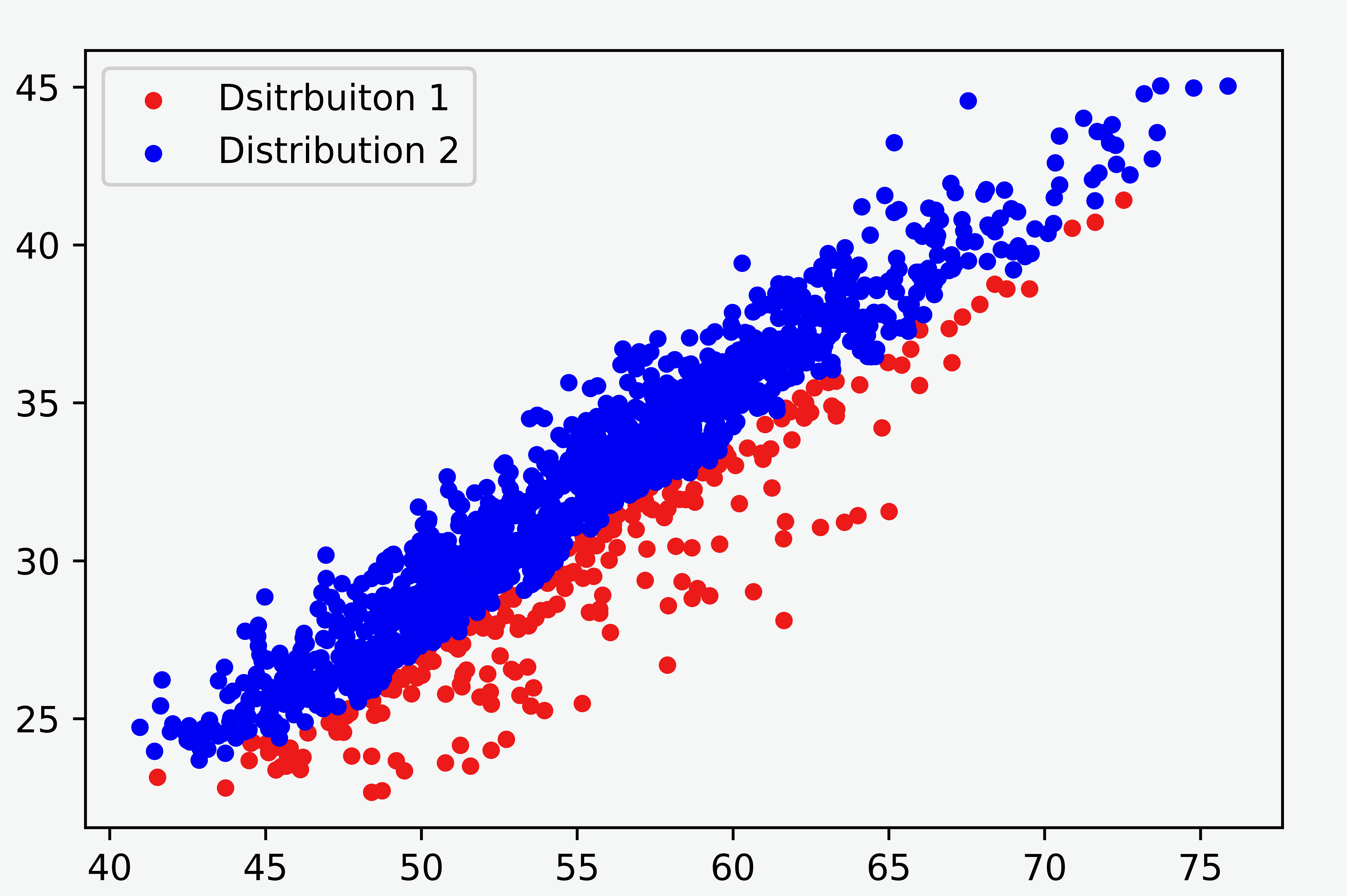
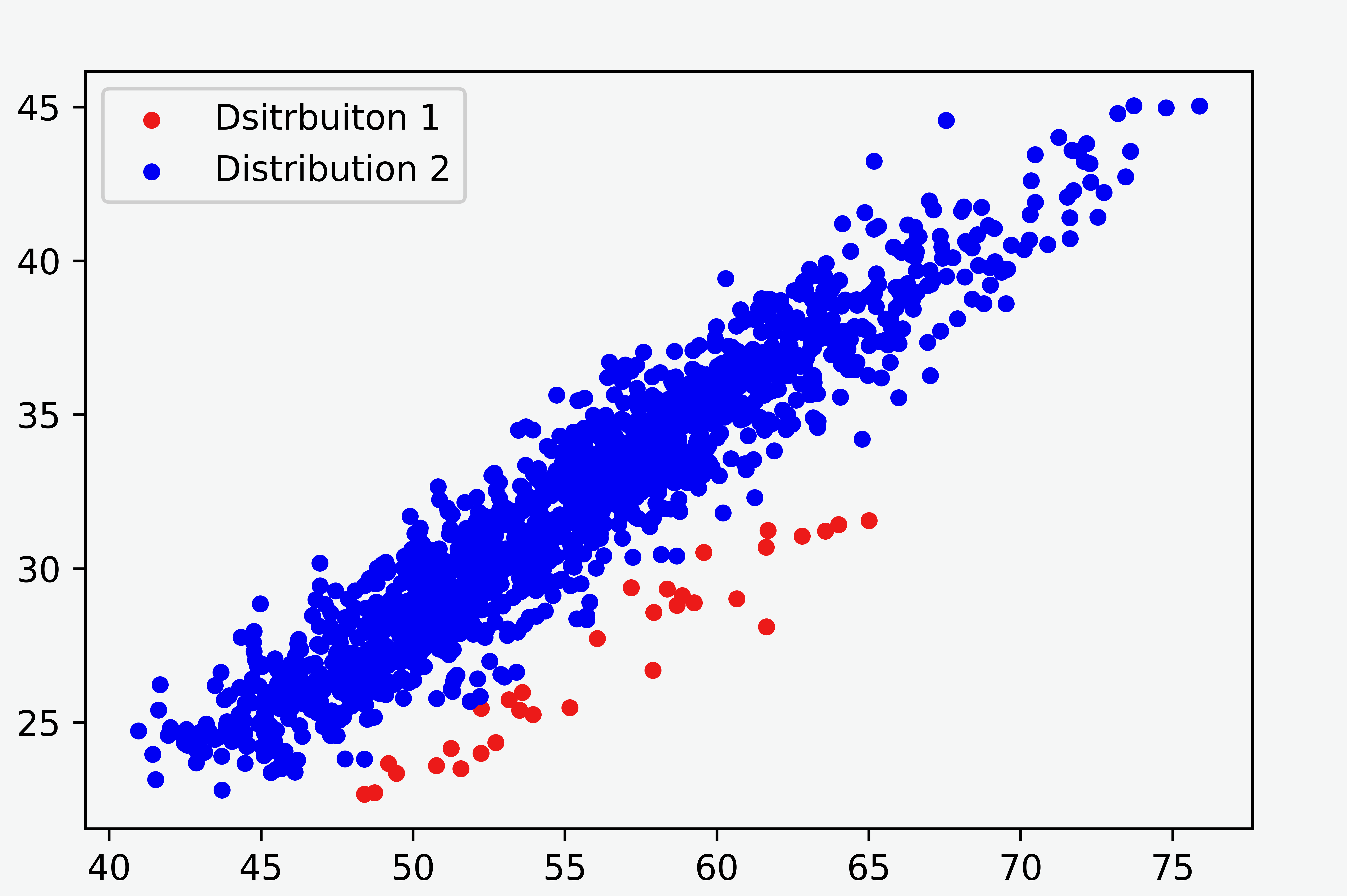
In this note, we compare the Gaussian mixture model and Student’s-t mixture model for some two-dimensional data with an unbalanced proportion of clusters, as shown in Figure 1. The result demonstrates that the Student’s-t mixture model performs much better.
Dimension Reduction
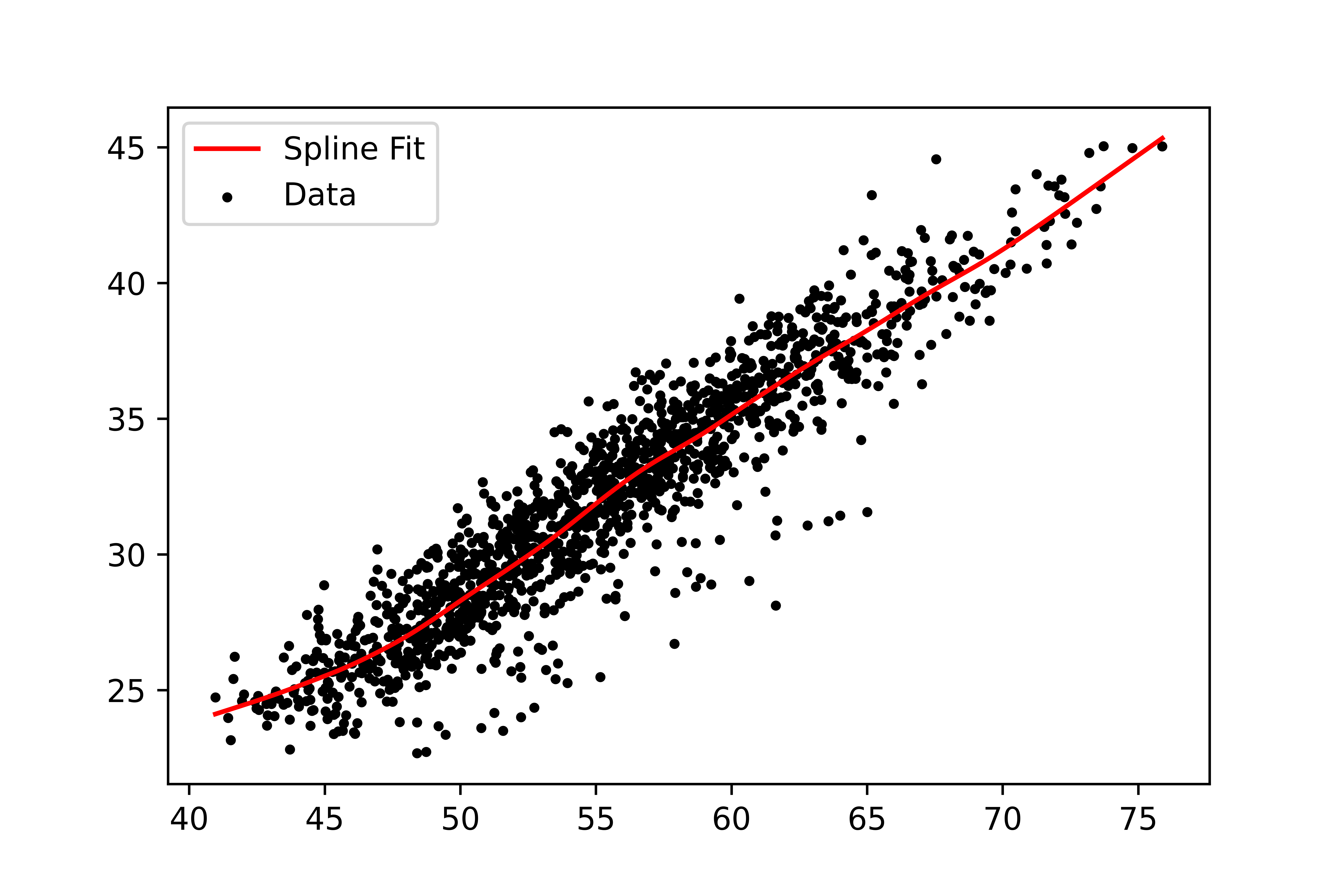
We first reduce the problem from two-dimensional to one-dimensional using spline fit since the variation between the clusters is mainly contained in the residual of the fit. We use the CSAPS package for Python to calculate the spline fit. The one-dimensional array of the residuals will be used for separating the groups with a mixture model.

Mixture Models
Gaussian Mixture Model
The Gaussian mixture model is widely used and assumes that the data are generated from mixtures of Gaussian distributions. We use GaussianMixure in scikit-learn with two covariance types: each component has its own covariance matrix (‘full’), and all components have the same covariance matrix (‘tied’).
Full Covariance Type
The result looks poor: it overestimates the difference in sigma but underestimates the difference in mean between the components. The sigma in one component is so large that the component is fragmented. The proportion of the smaller component is also too large.
| Component | Mean | Sigma | Fraction |
|---|---|---|---|
| 1 | -0.5 | 4.4 | 16.6% |
| 2 | 0.29 | 1.2 | 83.4% |
Tied Covariance Type
The result is improved by requiring the same covariance for all components: the fragmentation is gone. However, the result underestimates the mean difference, and the proportion of the smaller component is still substantial.
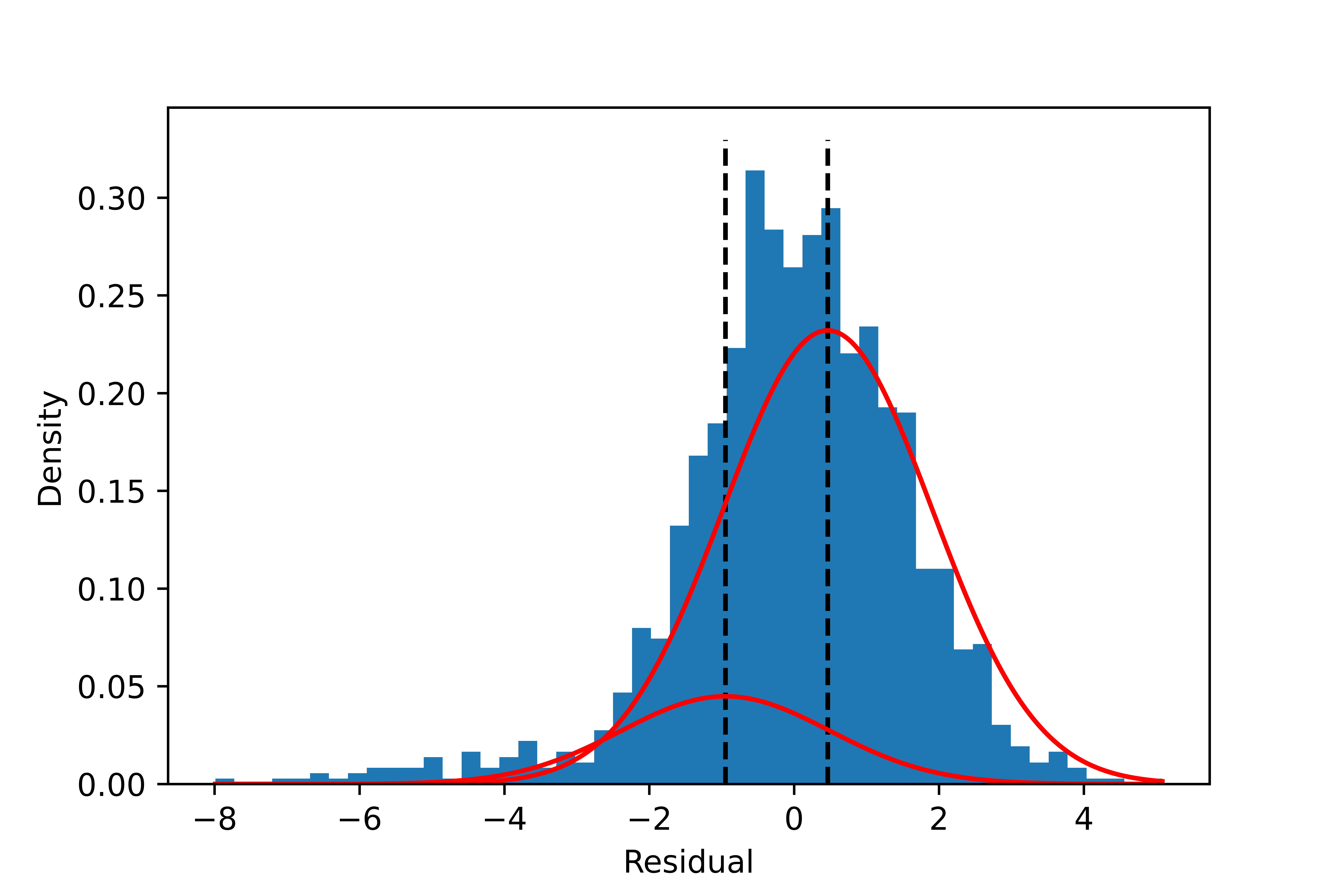
| Component | Mean | Sigma | Proportion |
|---|---|---|---|
| 1 | -0.95 | 2.1 | 16.2% |
| 2 | 0.46 | 2.1 | 83.8% |
Student’s t Mixture Model
To overcome the shortcomings of the Gaussian mixture model, we use Student’s t distribution (Equation ($\ref{eqn:student}$)) to model the components in the mixture model, described by Equation ($\ref{eqn:mixture}$).
\[p(x\mid\theta)=\sum_{k=1}^K \pi_k f(x\mid\mu_k, \sigma_k, \nu_k). \label{eqn:mixture}\]Student’s T distribution:
\[f(x\mid \mu, \sigma, \nu)=\frac{\Gamma\left(\frac{\nu+1}{2}\right)}{\Gamma\left(\frac{\nu}{2}\right)}\frac{1}{\sqrt{\pi\nu}\sigma}\left[1+\frac{1}{\nu}\left(\frac{x-\mu}{\sigma}\right)^2\right]^{-\frac{\nu+1}{2}}. \label{eqn:student}\]The Bayesian inference code with the PyMC3 package is listed below. Weakly informative priors are used.
def MixtureModel(data, nmode):
    """Inputs:
        data: 1-D array values
        nmode: integer, number of modes in distribution of data
       Output:
        model: PyMC model
    """

    ndata = len(data) # sample size

    with pm.Model() as model:

        p = pm.Dirichlet('p', a = np.ones(nmode), shape=nmode)

        #ordered mean
        mean = pm.Normal('mean', mu=np.ones(nmode), sigma=100, shape=nmode,
                         transform=pm.transforms.ordered, testval=np.arange(nmode))

        sigma = pm.Exponential('sigma', 1, shape=nmode)

        nu = pm.Exponential('nu', 1, shape=nmode)

        dist = pm.StudentT.dist(nu=nu, mu=mean, sigma=sigma, shape=nmode)

        obs = pm.Mixture('obs', w = p, comp_dists=dist, observed=data)

    return model

  ## Bimodal model, y is the residual array
  m2 = MixtureModel(y, 2)
  with m2:
    trace2 = pm.sample(1000, return_inferencedata=True)
  # Trimodal model
  m3 = MixtureModel(y, 3)
  with m3:
    trace3 = pm.sample(1000, tune=2000, target_accept=0.95, return_inferencedata=True)
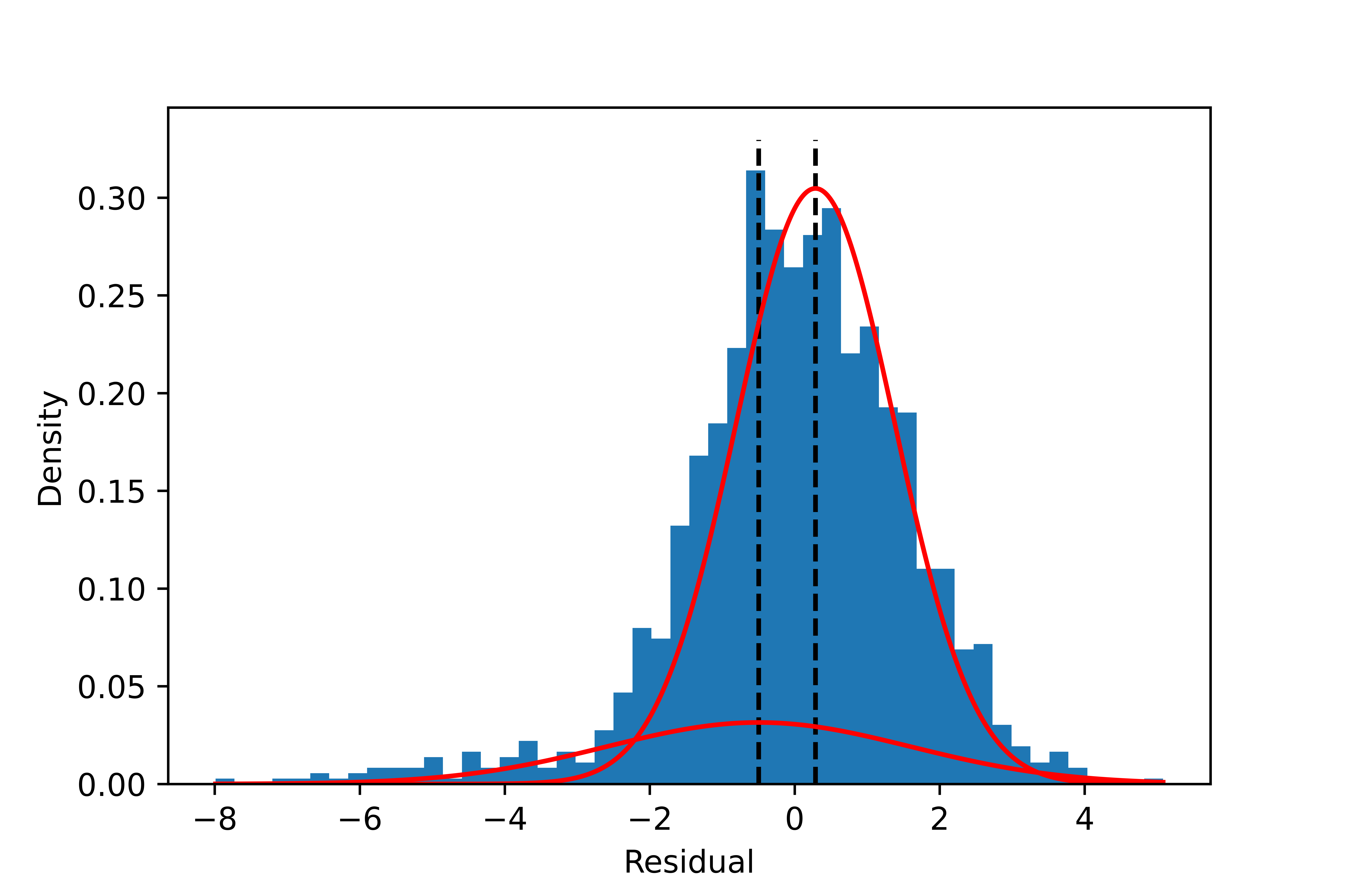
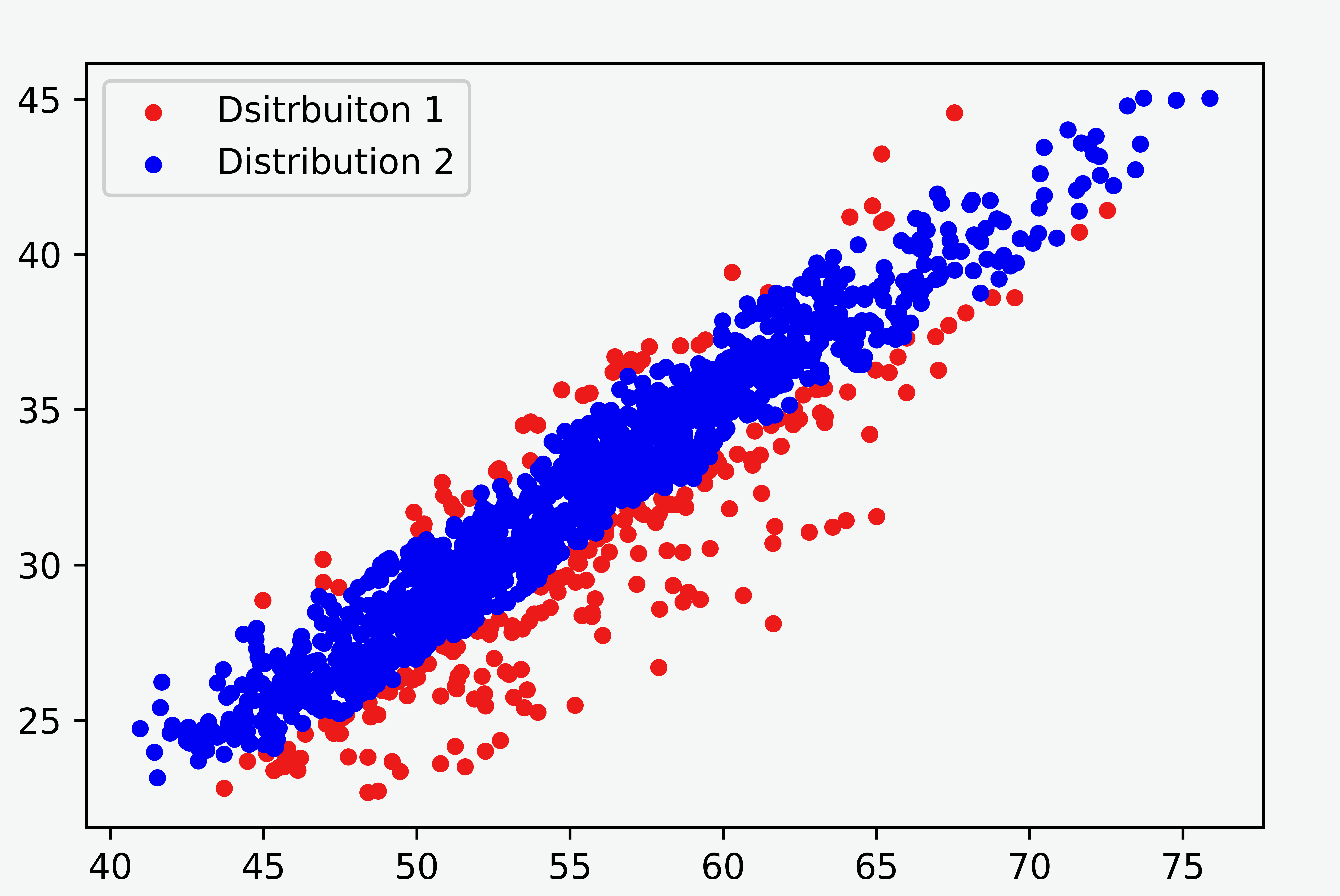
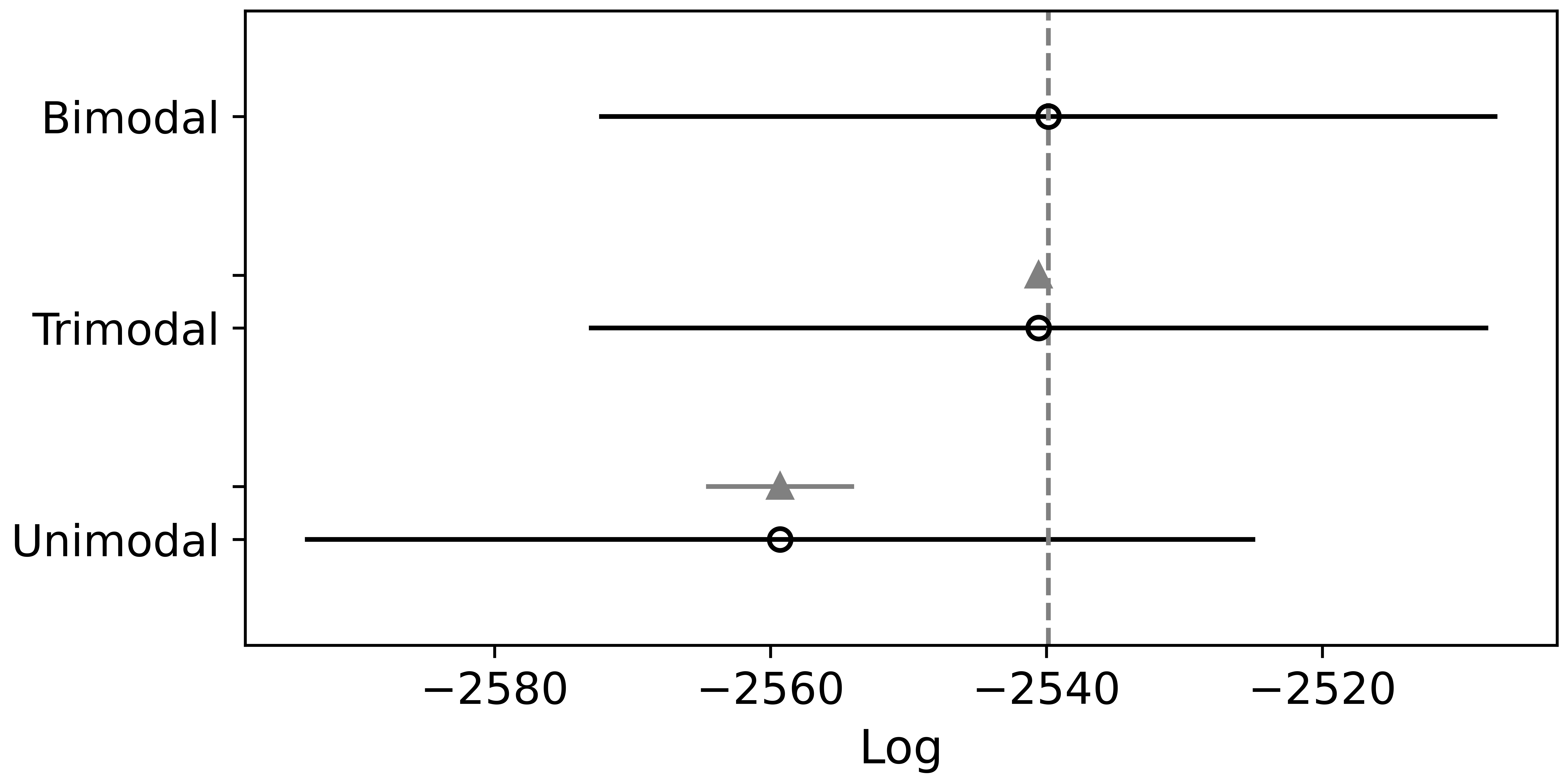
The model with two components is the best based on Pareto-smoothed importance sampling LOO cross-validation (Figure 5). As shown in Figure 6, The separation of the two components looks much better than with the Gaussian mixture model. The components’ location, spread, and proportions are also summarized in Figure 7 and the table below. They all have reasonable values.
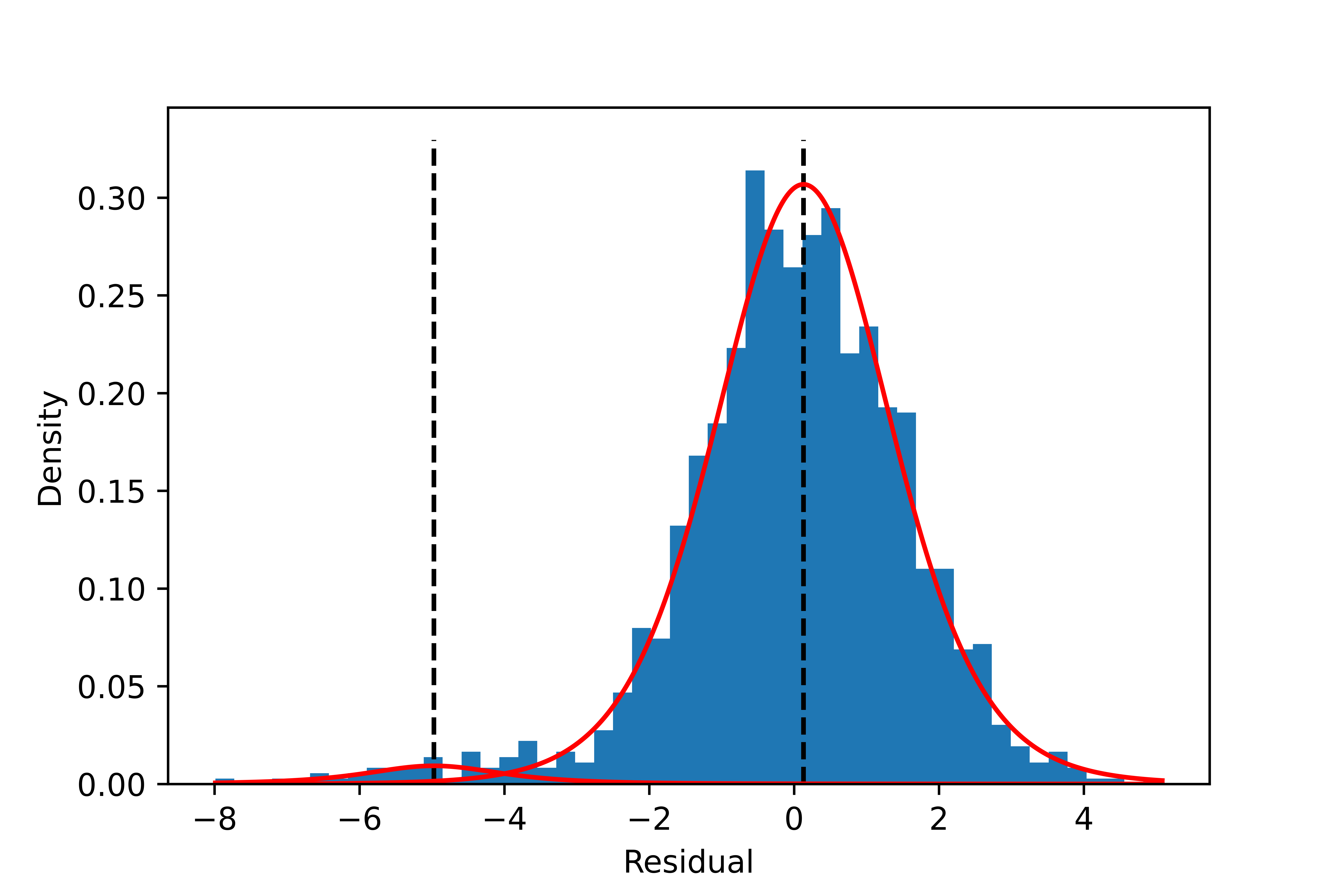
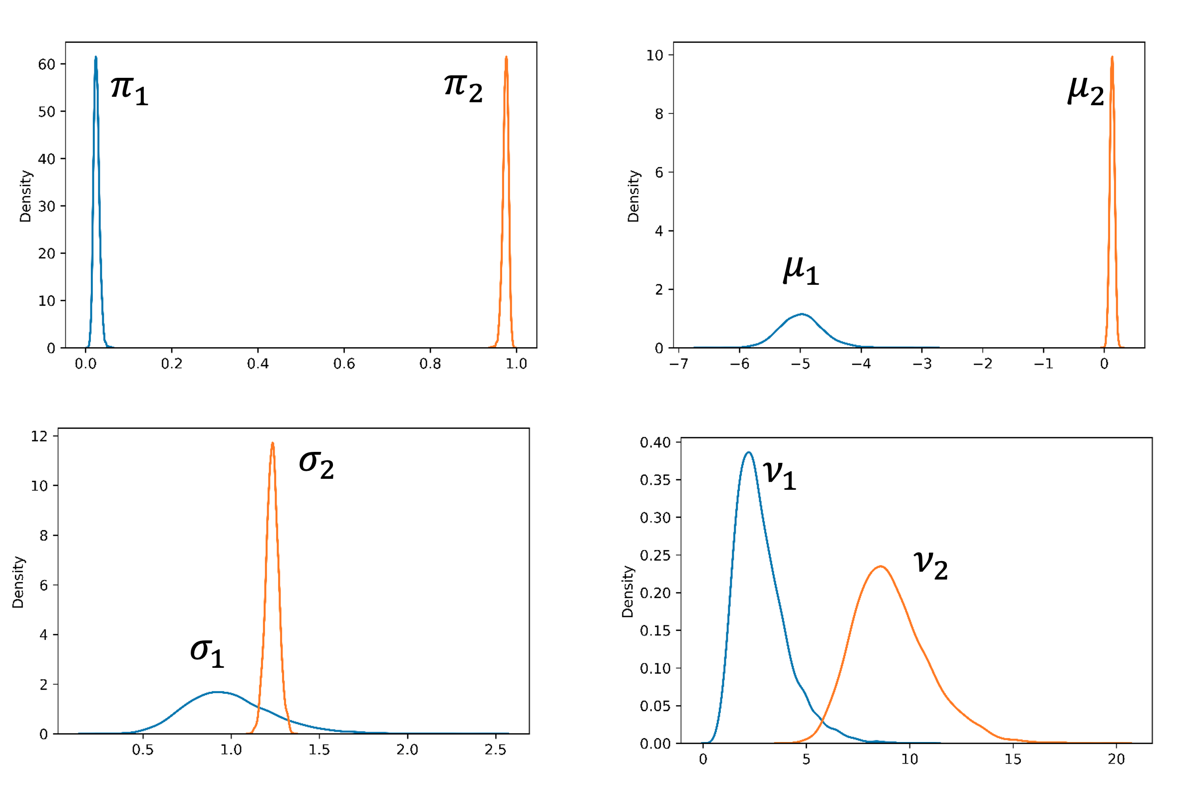
| Component k | Mean $μ_k $ | Scale $σ_k$ | nu $\nu_k$ | Fraction $π_k$ |
|---|---|---|---|---|
| 1 | -4.97 | 0.99 | 2.8 | 2.5% |
| 2 | 0.13 | 1.23 | 9.1 | 97.5% |
To summarize, the Student’smixture model is more robust than the Gaussian mixture model to handle imbalanced components and distributions with long tails. MCMC Bayesian inference using probabilistic programming packages like PyMC3 is straightforward to implement, and the result provides an uncertainty estimate through the posterior distributions.